Rotating Fourier Series
Chapter 12. Fourier Series Classically
Chaptere 12.1 Introduction
Actually, all the formulas related to the Fourier Series are presented in Fig. 7.2 in Chapter 7. They were based on the fact that the nth harmonic was a doubled vector indicating the nth centroid scn of the trajectory F(njω0t)=f(t)*exp(njω0t). More precisely, it was the complex amplitude of the nth harmonic of the f(t).
Now I will present formulas in the forms most often found in the literature, i.e.
-complex version with positive pulsations–>Ch. 12-6
-trigonometric version with positive pulsations–>Ch. 12-7
-complex version with positive and negative pulsations–>Ch. 12-8
-trigonometric version with positive and negative pulsations–>Ch. 12-9
Most often, Fourier Series lectures start with trigonometric formulas and only then move on to the complex version. For me it’s the opposite and probably more intuitive. I start from F(njω0t) with centroids scn, i.e. in the complex version and finish classically-trigonometrically.
Chapter 12.2 Relationship of the centroid scn of the trajectory with the nth harmonic
All 4 versions from the Introduction result, of course, from the nth centroids scn of the trajectories
in Fig. 7-2 of Chapter 7.2. The most important formulas that have happened in my life and are understandable. 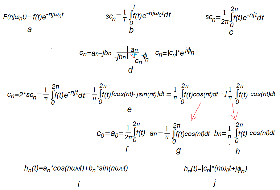
Fig. 12-1
Relationship of the centroid scn of the trajectory F(njω0t) with the complex Fourier coefficients c0, cn=an-jbn and harmonics hn(t) of the function f(t).
Fig. 12-1a
Trajectory F(njω0t)
Fig. 12-1b
General formula for the centroid scn of the nth trajectory F(njω0t) for f(t) with any pulsation n*ω0 or period T.
Fig. 12-1c
A more convenient formula for scn of the trajectory is when ω0=1/sec (i.e. T=2π sec).
This is almost, with some reservations, the general formula–> see Chapter 7.6.
Fig. 12-1d
nth Fourier coefficient as a complex number in different versions
Fig. 12-1e
nth Fourier coefficient as doubled centroid scn of nth trajectory F(njω0t).
It is shown how the coefficient was decomposed into cosine and snusoidal components. Differently – real and imaginary.
Fig.12-1f
The formula for the constant component is the coefficient of c0=a0 of the Fourier Series.
Fig. 12-1g
The formula for the an, or cosine, component of the Fourier Series. Red arrow shows “origin”
Fig. 12-1h
The formula for the bn, or sine, component of the Fourier Series. Red arrow shows “origin”
Fig. 12-1i
nth harmonic hn(t) as the sum of the cosine and sine components.
Fig. 12-1j
nth harmonic hn(t) as cosine with phase shift ϕ. Module |cn| is “Pythagoras” with an and bn.
Chapter 12.3 Test function f(t) for testing Fourier Series
We will find the Fourier Series for:
f(t)=0.25+1cos(1t)+0.3sin(1t)+0.6cos(2t)-0.4sin(2t)+0.4cos(3t)+0.2sin(3t).
Cosine and sine harmonics are visible. The Fourier Series formulas should confirm them. Then we will generalize the formula to any periodic function f(t).
Fig. 12-2
f(t)=0.25+1cos(1t)+0.3sin(1t)+0.6cos(2t)-0.4sin(2t)+0.4cos(3t)+0.2sin(3t) with pulsation period T=2π sec
c0=a0=+0.25 constant component
cn=an-jbn i.e when n=1,2,3
c1=1-j0.3 i.e. a1=+1 and b1=+0.3
c2=0.6+j0.4 i.e. a2=+0.6 and b2=-0.4
c3=0.4-j0.2 i.e. a3=+0.4 and b3=+0.2
Chapter 12.4 Sum of cosines and sines as rotating vectors
From chapter 2 Fig. 2-3 shows that the rotating vector exp(1j1t):
-is a two-dimensional model of the function f(t)=cos(1t)
-the projection of the rotating vector exp(1j1t) onto the real axis Re z is a function f(t)=cos(1t)
Similarly to chapter 2 Fig. 2-4 shows that the rotating vector -j*exp(1j1t):
-is a two-dimensional model of the function f(t)=sin(1t)
-the projection of the rotating vector exp(-1j1t) onto the real axis Re z is a function f(t)=sin(1t)
The above can be generalized, for example, into the three vectors from Fig. 12-3c rotating at speeds 1/sec, 2/sec and 3/sec and the appropriate linear combination of cosines and sines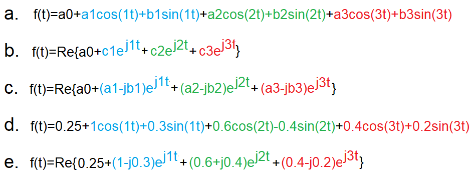
Fig. 12-3
a. Function f(t) as a linear combination of cos(1t),cos(2t),cos(3t) and sin(1t),sin(2t),sin(3t) and the constant a0.
b. Function f(t) as a projection of the rotating vectors c1*exp(1j1t), c2*exp(2j1t) and c3*exp(3j1t) and the constant a0 on the real axis, i.e. f(t)=Re{a0+…}
c. Rotating vectors with initial states c1=a1-jb1, c2=a2-jb2 and c3=a3-jb3 and the constant a0 are a model of the function f(t) from Fig a. Associate the parameters an and bn with the coefficients an at cosines and bn at the sines in Fig. a.
d. The specific case of the function when f(t) is from Fig. 12-2
e. Rotating vectors for the specific function in Fig. 12-2 as its model.
Fig.12-4
f(t)=Re{0.25+1cos(1t)+0.3sin(1t)+0.6cos(2t)-0.4sin(2t)+0.4cos(3t)+0.5sin(3t)
Interpretation of an animation lasting T=2πsec
+0.25 stationary vector, i.e. constant a0=+0.25
+(1-0.3j)exp(1j1t) first harmonic vector rotating at 1ω0=1/sec. In time T=2πsec it will make 1 revolution
+(0.6+0.4j)exp(2j1t) second harmonic vector rotating at 2ω0=2/sec. In time T=2πsec it will make 2 revolutions
+(0.4-0.2j)exp(3j1t) third harmonic vector rotating at 3ω0=3/sec. In time T=2πsec it will make 3 revolutions
And what will be the projections of these vectors in time? Return for a moment to Chapter 2.6 where you will find out that:
Re (a-jb)*exp(jω0t)=a*cos(ω0t)+b*sin(ω0t).
That is
Re (1-0.3j)exp(1j1t)=1cos(1t)+0.3sin(1t)
Re (0.6+0.4j)exp(2j1t)=0.6cos(2t)-0.4sin(2t)
Re (0.4-0.2j)exp(3j1t)=0.4cos(3t)+0.2sin(3t)
and
Re {+0.25}=+0.25 which is obvious
That is, the sum of the projections of rotating vectors on the Re axis is a function of f(t) from Fig. 12-2!
Or whatever comes to the same thing
The projection of the sum of rotating vectors onto the Re axis is a function of f(t) in Fig. 12-2!
Otherwise
The real part, i.e. Re of the sum of the sum of all rotating vectors on the Re axis, is the function f(t) from Fig. 12-2!
Chapter 12.5 Rotating vector as a model of the function f(t)=an*cos(n*ω0t)+bn*sin(n*ω0t)
When, for example, n=1 and ω0=1/sec then a1=1, b1=-0.3 i.e. f(t)=1*cos(1t)+0.3*sin(1t)
Fig. 12-5
Rotating vectors as a model of the function f(t)=1cos(1t)+0.3sin(1t)
Fig. 12-5.1
Single rotating vector as f(t) model
a. Rotating vector +(1-0.3j)*exp(1t)
b. f(t)=Re{(1-0.3j)exp(1j1t)}
Otherwise, the projection of the rotating (1-0.3j)*exp(1j1t) on the real axis Re z is a function f(t)
Fig. 12-5.2
A pair of contrary rotating vectors as a model f(t)
a. Rotating vector+(0.5-0.15j)*exp(1t). This is one-half of the rotating vector in Fig. 12-5.1a
b. Above rotating vector but in the opposite direction +(0.5+0.15j)*exp(-1j1t).
As a complex number, it is at any moment a conjugate number with respect to the rotating vector a.
Note
Complex numbers, e.g. z=5+3j and z*=5-3j, are so-called conjugate numbers. Note that z* is a mirror image with respect to z when the “mirror” is the real axis Re z.
c. f(t)=(0.5-0.15j)*exp(1t)+(0.5+0.15j)*exp(-1j1t)
In other words
The sum (complex or vector) of oppositely rotating vectors a and b is a real function f(t).
Indeed, vector b on Fig. 12-5.1b moves identically to vector c on Fig. 12-5.2b. Note that we do not need to derive the function f(t) as the real part of a complex number!
Conclusions
1. Both models, i.e. a single rotating vector and a pair of rotating vectors, describe the same function f(t), i.e.
f(t)=an*cos(n*ω0t)+bn*sin(n*ω0t)
2. Single rotating vectors are used in Chapter 12.6 Complex Fourier Series with Positive Pulsations
3. Pairs of rotating vectors are used in Chapter 12.8 Complex Fourier Series with Positive and Negative Pulsations
Chapter 12.6 Complex Fourier Series with Positive Pulsations
This is a generalized formula for single rotating vectors from Fig. 12-3e and the animation of Fig. 12-4 for n=∞
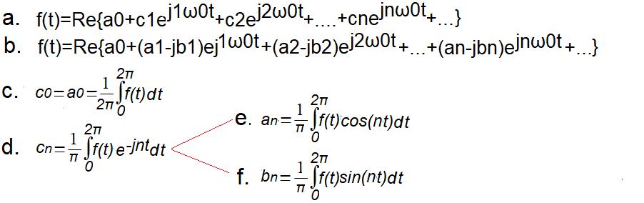
Fig. 12-6
Complex Fourier Series with positive pulsations
Any (almost, but let’s not go into details) periodic function f(t) can be represented as an infinite series of rotating vectors plus a constant component co.
a. Single rotating vectors with complex amplitudes c1, c2 …cn with a constant component c0. The projection of these vectors onto the real axis Re z (i.e. Re{…} is the function f(t). The speed ω0, e.g. ω0=1/sec, corresponds to the pulsation of the periodic function f(t).
b. As above, only complex amplitudes as c0=a0, c1=a1-jb1, c2=a2-jb2,…cn=an-jbn
For example, for the animation in Fig. 12-4
a0=+0.25
c1=a1-jb1=1-j0.3–>a1=1 b1=+0.3
c2=a2-jb2=0.6+j0.4–>a2=0.6 b2=-0.4
c3=a3-jb3=0.4-0.2j–>a3=0.4 b3=+0.2
c. Formula for the constant component c0=a0 of the periodic function f(t).
d. Formula for complex coefficients cn of the periodic function f(t), in other words for complex amplitudes cn for nth harmonics.
This is the doubled centroid scn of a rotating trajectory with speed n*ω0.
You can take it on your word of honor, but they should convince you
– chapter 7 theory
– chapter 11“Checking patterns…”
I advise you to read the commentary to Fig. 12-1c.
e. real component, complex amplitude an, also known as cosine
f. the imaginary component of the complex amplitude bn, also sine
Note that ω0, i.e. the fundamental pulsation of the function f(t), appears only in formulas a and b. However, they do not appear in formulas d, e, f. The coefficients an, bn, e.g. of a square wave, depend only on its amplitude and duty cycle. However, they do not depend on its pulsation, frequency or period. I wrote about it in chapter 7.6.
Chapter 12.7 Trigonometric Fourier Series with Positive Pulsations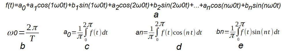
Fig. 12-7
Trigonometric Fourier Series with positive pulsations
a. Fourier Series with positive pulsations.
It follows directly from the formulas
– Fig. 12-6b where f(t) is the real part of the complex function in braces Re{…}
In other words, the complex function in the braces is the sum of rotating vectors (an-jbn) and the projection of this sum is the function f(t).
b. Pulsation of the first harmonic ω0 where T is the period of the function f(t)
c. Constant component a0
d. nth cosine component an
e. nth sinusoidal component bn
Chapter 12.8 Complex Fourier Series with Positive and Negative Pulsations
The Fourier Series is based on the centroids scn of trajectories F(njω0t) rotating at speeds n*ω0. They are the complex amplitudes for these pulsations. Previously, i.e. in chapters 12.6 and 12.7 were doubled amplitudes.
Section 12.8.1 Complex Fourier Series with positive and negative pulsations for the test function f(t).
If in the formula Fig. 12-3e and in the animation Fig. 12-4 we replace each individual rotating vector with a pair of rotating vectors, we will obtain the animation below. For example, the single rotating vector of Fig. 12-5.1 has been replaced by a pair of rotating vectors of Fig. 12-5.2.
Fig. 12-8
f(t)=(0.2+0.1j)*exp(-3jt)+(0.3-0.2j)*exp(-2jt)+(0.5+0.15j)*exp(-1jt)+0.25+(0.5-0.15j)*exp(+1jt)+(0.3+0.2j)*exp(+2jt)+(0.2-0.1j)*exp(-1jt).
The 3 left vectors rotates opposite to the 3 right ones and form 3 pairs of oppositely rotating vectors. The central vector +0.25 does not rotate and is the constant component a0 of the function f(t). The function f(t) is the sum of the above rotating vectors. Unlike Fig. 12-4 (with the same f(t)!), there is no need to use the real part dereference operation of f(t). Instead of f(t)=Re{…} we simply write f(t)=…
Someone may wonder. On the right side of the equation are rotating vectors, and on the left is the real function f(t). As if there were pears on the right and cows on the left. So let’s sum the right vectors (including the constant vector a0=+0.25, more precisely a0=(0,+0.25). We will get the left pulsating vector with a constant component a0=+0.25, which is f(t)!
Fig. 12-9
The pulsating vector as f(t) as the sum of the rotating vectors of Fig. 12-8
a. A vector pulsating on Re z from the real axis with a constant component a0
b. Function f(t) describing the motion of the pulsating vector on the Re z axis
This is exactly the function of Fig. 12-2. On the left side of the equation Fig. 12-4 there is also the same function f(t), but on the right there is the projection of the sum of rotating vectors, i.e. Re of {…}.
Let’s get back to the topic again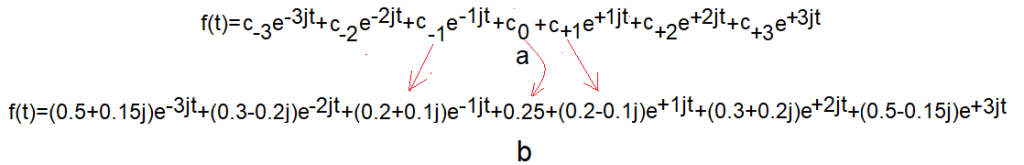 Fig. 12-10
a. Complex Fourier Series with positive and negative pulsations of c(n) coefficients for n=0…+∞.
b. Example of a Complex Fourier Series with positive and negative pulsations and specific complex coefficients c(n) for n=0,1,2,3.
e.g. c(-1)=0.2+0.1j, c(0)=+0.25, c(1)=0.2-0.1j
Note that e.g. c(-1) is the conjugate of c(1)
We obtained the coefficients a(n),b(n) for positive and negative n directly from formula 12-10b. They did not need to be calculated (although they could be).
Chapter 12.8.2 Complex Fourier Series with positive and negative pulsations for any function f(t).
This is the formula we obtain by generalizing Fig. 12-10a. By the way, something cool will come out. A Fourier series with only positive pulsations has complex harmonic amplitudes, they are double the centroids of the scn of the rotating trajectories F(njω0). Now we know why scn were previously doubled. Because they handled 2 times less harmonics.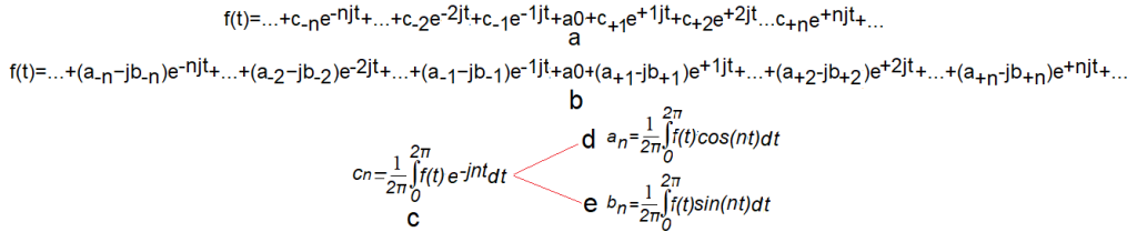
Fig. 12-11
a. Complex Fourier Series with positive and negative pulsations with coefficients cn
b. Complex Fourier Series with positive and negative pulsations with detailed coefficients cn
Note that each Fourier coefficient c(+n)=a(n)-jb(n) at positive pulsations nω0 corresponds to a Fourier coefficient c(-n)=a(-n)+jb(-n). These coefficients are conjugate numbers c(+n)=c(-n)*
c. formula for the complex c(n) Fourier coefficient. It is 2 times smaller than the corresponding coefficient c(n) on the Fourier Series in Fig. 12-6d
d. formula for a(n)=a(-n)
e. formula for b(n)=-b(-n)
Note that the coefficients c(n), a(n) and b(n) are 2 times smaller than the c(n), a(n) and b(n) in chapter 12.6.
Chapter 12.10 Trigonometric Fourier Series with positive and negative pulsations.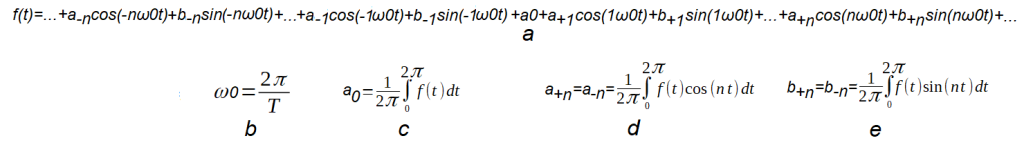
Fig. 12-12
Trigonometric Fourier Series with positive and negative pulsations
a. Fourier series with positive pulsations.
It follows directly from the formulas
– Fig. 12-11b where f(t) is the real part of the complex function in braces Re{…}
– Fig. 2-9d chapter 2
b. Pulsation of the first harmonic ω0 where To is the period of the function f(t)
c. Constant component a0
d. formula for a(n)=a(-n)
e. formula for b(n)=-b(-n)
Note that the coefficients a(n) and b(n) are 2 times smaller than a(n) and b(n) in the chapter. 12.7
Chapter 12.11 Trigonometric Fourier Series with positive and negative for arbitrary T.
Often, the coefficients an, bn do not depend on the period T of the function f(t). For example, for a square wave with 50% duty cycle, they are the same for the period T=1 sec and T=3 sec. Then we can assume that Tπ=2π as in Fig. 12-12. It’s always one parameter less and easier calculations. See chapter 7.7. But this is not always the case. You will find out about this in the article “Fourier Transform” chapter. 3.3. Then we use the formula with “general T”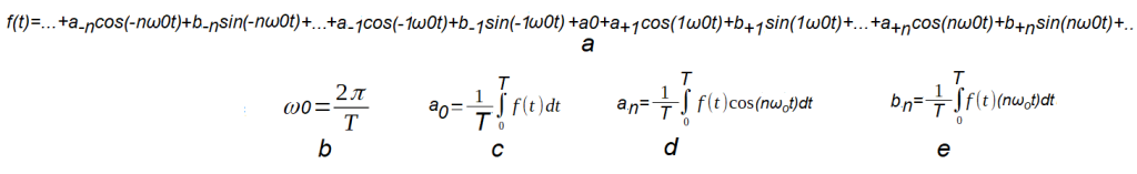 Fig. 12-13
Trigonometric Fourier series with positive pulsations for the interval T/2…+T/2.
Such a range can sometimes make our calculations easier.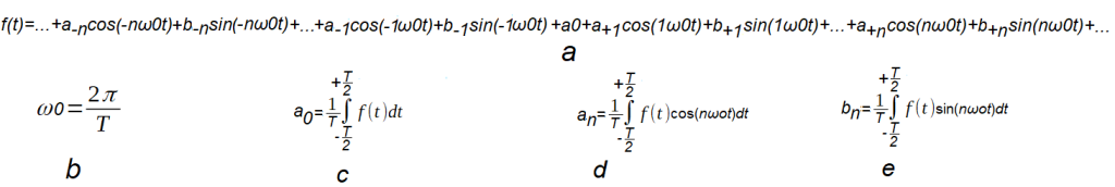
Fig. 12-14
Trigonometric Fourier series with positive and negative pulsations for the interval 0…T or -T/2…+T/2.
Such a range can sometimes make our calculations easier.