Automatics
Chapter 22 Continuous Control
Chapter 22.1 Introduction
Fig. 22-1
Fig. 22-1a
The most general control diagram showing:
– setpoint x(t)
– output signal y(t) –other name process variable
– disturbance z(t)
– control error e(t)
Fig. 22-1b
A more accurate version in which the entire G(s) object has been divided into an ON/OFF controller and the proper Go(s) object. The control signal s(t) appeared after the controller.
Fig. 22-1c
Instead of a ON/OFF controller, there is a P, PI, PD or PID continuous type controller.
The control signal s(t), unlike the ON/OFF controller, is continuous.
Chapter 22.2 General and typical form of the Go(s) object
From now on, we are only interested in continuous control, i.e. Fig. 22-1c. But first, let’s deal with the object itself, which will be controlled by the controller. The Go(s) examples are: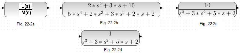
Fig. 22-2
Fig. 22-2a
General form of the G(s) transmittance where the numerator L(s) and the denominator M(s) are polynomials.
Fig. 22-2b
Specific example where the numerator L(s) is a polynomial of degree 2 and the denominator M(s) of degree 4.
Fig. 22-2c
Cases of Go(s) object transmittance when L(s) is of degree greater than 1 are rather rare! A typical numerator L(s) is only the gain K. Here K=10.
Fig. 22-2d
In turn, most often K=1 and we will treat this transmittance as typical. The denominator M(s) is still a polynomial of any degree n. Often M(s) is a product of.. E.g. M(s)=(1+sT1)(1+sT2)(1+sT3) 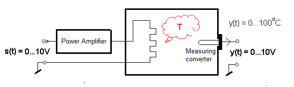
Fig. 22-3
An example that K=1 is typical as in Fig. 22-2d
The Go(s) object is a water tank with a resistance heater controlled by a power amplifier. The water temperature will be controlled in the range of 0…+100ºC. We measure it with a Pt100 resistance thermometer with a measuring range of 0…+100ºC–>voltage 0…+10V. The thermometer consists of a platinum wire in a metal casing-tube and a ΔR–>0…10V converter. ΔR is the increase in resistance R due to an increase in temperature. The tube with the wire is quite delicate and therefore it is placed in a metal sheath. The transducer protrudes outside the tank, from where the signal can be connected with a cable to the controller. In the picture you can see how the sheath enters the tank through the hole.
The power amplifier is tuned so that +10V per input will heat up to +100ºC, but without boiling! Also the temperature transducer will give +10V. And when it is not possible to achieve this value,but for example +55ºC? Now you need to increase the boiler power by increasing the power of the amplifier.
When s(t)=0…+10V then s(t)=0…+10V. That is relationship between s(t) and y(t) is like the Ko=1 amplifier. Of course, with time constants T which are included in the transmittance denominator Go(s). The degree of the M(s) polynomial is the greater the more accurately we know the mathematical description of the water heating process in the tank. The simplest approximation, is an inertial unit.
Conclusion
The Go(s) object is a water tank + heater + power amplifier. Gain of the object itself Ko=1. And what if in front of the object, i.e. in front of the power amplifier, there is an ordinary voltage amplifier (not power amplifier!) with a gain of e.g. Kp = 5? Later you will learn that this amplifier is a proportional controller, or in other words, a P controller. Then the gain of the entire open circuit is K=Kp*Ko=Kp, because Ko=1, so it depends only on the setting of the P controller – gain Kp. And this will facilitate the so-called regulator tuning. That is, finding a Kp that will provide the optimal response to the step unit x(t).
Chapter 22.3 Static and astatic Go(s) objects.
The automatics engineer begins the project with a good knowledge of the Go(s) objects he is to control, i.e. its static and dynamic properties.
These are:
-static
-astatic
Chapter 22.3.1 Static objects.
You are examining the simultaneous response to a step x(t) of three typical static objects
Fig. 22-4
G1(s)-Inertial unit K=1 T=2sec
G2(s)-Double Inertial unit K=1, T1=2sek, T2=3sec
G3(s)-Oscillation unit K=1, q=0.3, T=1sec –>chapter.7 Fig. 7-2
In steady state, all outputs in response to x(t) are constant, i.e. static. Hence the name static objects. Note that each denominator M(s) of the transmittance G(s) does not have a zero root.
Chapter 22.3.2 Astatic objects
Simultaneous response to a step x(t) of three typical astatic objects.
There are zero roots in the denominator M(s). Even double–>G2(s).
Fig. 22-5
G1(s)-Integral
G2(s)-Double Integral
G3(s)-Integral with inertia
In steady state, the outputs y(t) keep increasing! y1(t), y3(t) at a constant speed. For y2(t) even better, with the speed that is increasing all the time – like after the start of the Apollo rocket! This is typical for astatic objects, i.e. non-static. That is, those that, in response to a step x(t) in a steady state, move with a constant or with an increasing speed. A characteristic feature of these objects is also a non-zero output with zero input in a steady state. This feature ensures precisely zero control error is related to the I component of the PID controller. This will be discussed later.
Interpretation
G1(s) – an ideal DC motor with a gear and a lever. So, in our way, actuator. The input is the voltage on the motor, the output is the angle α. This α can control, for example, a valve in the pipeline. I emphasize that there is no negative feedback here, i.e. the angle can change theoretically from – to + infinity. In practice, the engine will be switched off earlier by the so-called limit switches. And even earlier it is turned off or even “turned back” by the regulator providing negative feedback.
G3(s) – Same thing, just an imperfect actuator. That is, taking into account inertia and friction. Hence the acceleration effect before it reaches a constant speed.
G2(s) – Rocket as above, or an actuator that increases speed all the time!
The latter is a purely theoretical case, rather not used in practice. Or maybe they are?
An astatic object can only be stopped by giving zero to the input.
Even more trivial.
With a non-zero input x(t):
Static in a steady state, it does not move.
Astatic in a steady state it moves.
Chapter 22.4 Comparison of static and astatic objects due to stability
Chapter 22.4.1 Introduction
It is probably easier to control something that does not move in a steady state than something that moves.
Therefore, static objects are “easier” than astatic ones. Let’s check it.
Chap. 22.4.2 Static
A typical 2nd degree static object with negative feedback.
Fig. 22-6
The system reached a steady state y=0.91. It is the fixed error, here e=0.09, the smaller the greater the gain K, is typical for static systems with negative feedback. If you want to reduce the error, you need to increase K. However, this will cause greater oscillation and sometimes even instability. It can be proved, for example, from the Nyquist criterion that systems of the two-inertial type will never become unstable, even with a large K. Because their amplitude-phase characteristics only pass through 2 quadrants. Only those transmittances whose denominator degree M(s) is greater than 2 can enter instability.
Chap. 22.4.3 Astatic
Astatic ones are more difficult to control because they become unstable more easily when closed with negative feedback.
Fig. 22-7
The zero root s=0 in the denominator M(s) of transmittance appeared. A typical feature of astatic systems. Let’s give 5 seconds for the input “click” x(t). I already know what will happen. Therefore, I radically changed the scale of the oscilloscope. Previously it was 0…+1.2, now -150…+150. Misfortune. Instability, oscillations from – to + infinity. And only the small letter s in the transmittance in Fig. 22-7 did it.
And how to make the system stable? Generally, it does different things. The first thought is to reduce K.
It will be quite a radical reduction from K=10 to K=0.25.
Fig. 22-8
The most important is that the answer is stable. But how slow! Compare with Fig. 22-6, where the steady state occurred after approx. 10 seconds, here after 55 seconds. But there is one nice thing about it. After 45 sec. we have the state y(t)=x(t). So zero error! And that’s regardless of K! For example, K=0.1, the fixed error would also be zero. Unfortunately, at the expense of slow time charts,
That is, astatic objects with negative feedback are more susceptible to oscillations and instability. They are also slower to reach a steady state. However, they can reduce the error to zero, which is of course their main advantage.
Chapter 22.4.4 Comparison of static and astatic with feedback in a common graph
We will compare the respones with:
-Fig. 22-6 (static stable)
-Fig. 22-7 (astatic unstable)
-Fig. 27-8 (astatic stable).
In these figures, there were different oscilloscope settings for time t and y(t). Therefore, we will examine all 3 transmittances again, but this time simultaneously. 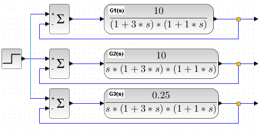
Fig. 22-9
Press start
The same step x(t) enters all 3 objects:
– G1(s) static
– G2(s) astatic – high gain K=10 therefore unstable
– G3(s) astatic – low gain K=0.25 therefore stable
Fig. 22-10
These vertical yellow lines are increasing oscillations of the object G2(s) with negative feedback. In Fig. 22-7 there was an answer to x(t)=dirac and now x(t)=step.
Conclusions:
– Astatic systems are more susceptible to instability than static ones
– Stable static system G1(s) clearly reaches a steady state faster than stable astatic G3(s)
– Stable astatic system G1(s) may have a zero error! Of course, provided that it is stable, which is more difficult for astatic ones. It is precisely this zero control error e(t) in the steady state that is the basic advantage of astatism.
Static systems, unlike astatic ones, provide zero error only for the gain K=infinity. This rather theoretical condition can cause large oscillations and even instability.
Chapter 22.5 Man as a Continuous Controller
Chapter 22.5.1 Introduction
A customer contacted us about the design of the control system for the facility shown in Fig. 22-3.
He is a poor investor and cannot afford a controller. He will do it for him himself, i.e. he will control it manually
About the facility itself, he only said:
– it is a tank with a liquid z which does not change state at all. This assumption will facilitate our analysis.
– wishes to control the temperature continuously in the range of 0ºC…+50ºC
He also cares about the fastest possible transition from one state to another, e.g. from +20ºC to +40ºC, or vice versa from +40ºC to +20ºC. The latter is associated with active cooling, i.e. the heater will turn into a refrigerator! Hence the cooling Peltier element.
And why should the controller be continuous and not ON-OFF? Because he knows that in a steady state for ON-OFF control, the output signal y(t) oscillates around a certain average value all the time. And this has a very bad effect on the quality of the customer’s product!
Chapter 22.5.2 Man as a Continuous controller without feedback
We proposed open-loop control, or if you prefer control without feedback.
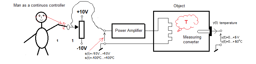
Fig. 22-11
It is almost repeated Fig. 22-3 with a man as a controller and a potentiometer as a direct control device. We already know about the object itself that changes in the voltage s(t)=0…+10V at its input correspond to the same changes y(t)=0…+10V at the output, but in a steady state! Strictly the same changes but only for s(t)=0…+5V. We just assumed that the output temperature will never exceed +50ºC and there is no point in giving the thermometer range 0… +100ºC.
So the whole complicated object with a boiler, liquid and thermometer has been reduced, even degraded to an ordinary amplifier with a gain of K=1 with certain T time constants. Because if there is e.g. +3V on the potentiometer, there will also be +3V on the steady-state output of the thermometer (meausuring converter)! This approach greatly facilitates the selection of a continuous controller PID type, in which the entire controller dynamics of the closed system will depend only on the Kp, Ti and Td settings of this controller. This will be discussed in the following chapters.
User manual
Our Client not only cannot afford the controller, but he is also an orphan–> he needs to be taught how to control it, i.e. give him an instruction manual.
1. It will control the potentiometer providing the voltage in the range -10V…+10V. It is 200 mm long and is calibrated in units of 0.1V<=>1ºC or 0.1mm<=>1ºC. It is 0ºC in the middle, +100ºC at the top and -100ºC at the bottom.
One more thing. This is an automatics course, not physics. Therefore, the liquid does not change state -> does not freeze or evaporate.
In addition, our electric boiler heats with positive voltages and cools with negative voltages! There is a freak known since the 19th century – the Peltier element.
The Client reads the manual with mixed feelings
He has at his disposal:
-control device–> potentiometer with a range of -10V…+10V, otherwise -100ºC…+100ºC
–temperature converter with a range of 0…+50ºC, otherwise 0…+5V
The Client is surprised. Should I control the temperature of the liquid in the range of 0…+50ºC? Why redundant “heating/cooling” power, e.g. -10 kW…+10kW, if 0…+5 kW is enough for 0ºC…+50ºC? Or maybe the designer wants to let me in on costs, like a taxi driver driving not the shortest route? Why do I need control enabling temperatures of -100ºC…+100ºC and the temperature transmitter range is only 0…+50ºC?
And so, with doubts, he proceeded to the first attempt to heat the liquid to +30ºC.
The first attempt to heat the liquid to +30ºC.
He approaches the problem as carefully as a dog to a hedgehog. Therefore, he moved the slider up by 30 mm to s(t)=+3V or, if you prefer, to +30ºC and waits for the effect. The Client blindly believes in the s(t) control slider and does not even look at the thermometer! I will add that the ambient temperature is 0ºC. The client’s faith had a basis. After some time, the temperature increased to +30ºC as shown below.
Fig. 22-12
You can see in the upper left corner how the Client moved the potentiometer slider from 0V to +3V after about 5 seconds, which corresponds to the temperature step from 0ºC to +30ºC. The step wasn’t perfect. Our Client is getting old and the paw is shaking a bit. Anyway, you can see how beautifully the temperature y(t) goes from 0ºC to +30ºC.
It was an example of absolutely open control. i.e. The Client didn’t even look at the thermometer, just trusted the control slider completely. The output signal y(t) had no effect on the control signal s(t) from the slider! And the time chart itself is a classic inertial unit with K=1 and T=10sec
Chapter 22.5.3 Man as a Continuous controller with feedback.
It would seem that open-loop control is great! The Client set the slider to s(t)=+3V=+30mm=+30ºC and after some time the temperature reached +30ºC What more could you want?
But
First
The ambient temperature was 0ºC. If it were otherwise, e.g. +13ºC, then in steady state it would be y(t)=+43ºC (actually a little less) and not y(t)=+30ºC!
Second
We assumed that the object the object has been identified mathematically and physically i.e. we know that at an ambient temperature of 0ºC and s(t)=+3V on the potentiometer, the temperature of the liquid should be set exactly at y(t)=+30ºC.
Thirdly
We assumed the potentiometer was perfect. i.e. that 30 mm up is exactly s(t)=+3V
Fourth, etc…
In short, we assumed everything was perfect. And these were just blissful wishes. So we cannot be sure that 30 mm up on the potentiometer will heat the liquid to exactly +30ºC. There can only be one conclusion.
The Client must constantly observe the output signal y(t) and correct it with the potentiometer slider.
So the diagram should look like this.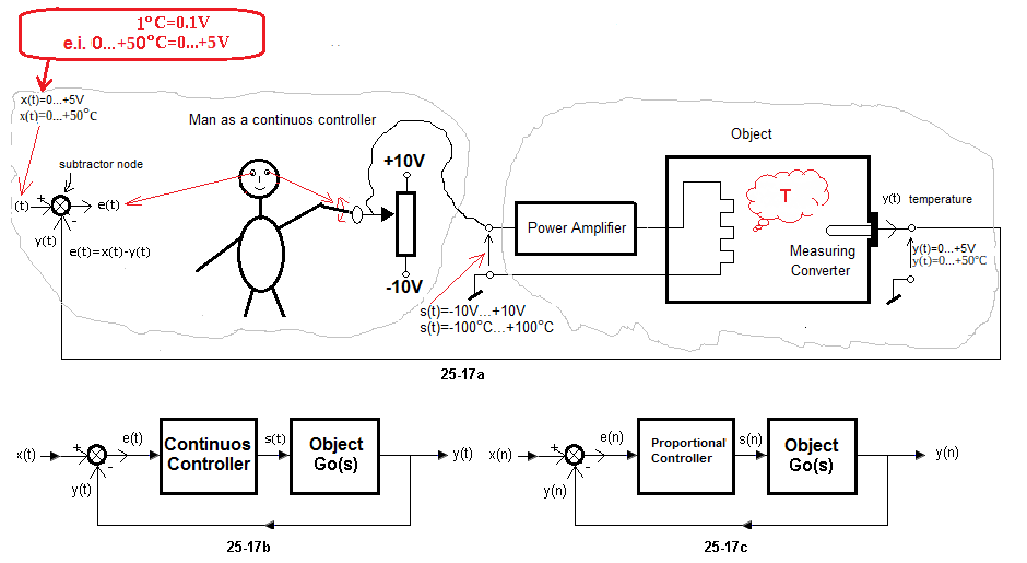
Fig. 22-13
Man as a Controller
Fig. 22-13a
The Client constantly observes the output signal y(t) and, depending on the situation, corrects it with the voltage signal s(t) from the potentiometer. So in the “head” he calculates the error e(t)=x(t)-y(t) and combines it so that the error e(t) in the steady state is as small as possible. The unachievable ideal is that e(t)=0 at any time. Then y(t)=x(t), i.e. the output signal y(t)=x(t). Otherwise–> y(t) tries to follow the set value x(t).
Fig. 22-13b
The Client used some algorithm to reduce the error e(t) to zero. It can also be performed by a microprocessor.
Then the man is replaced by the controller as above.
Fig. 22-13c
There are many such algorithms. One of them is surprisingly simple!
step 1 calculate the current control error e(t)=x(t)-y(t)
step 2 calculate the control signal s(t)=Kp*e(t)
step 3 return to step 1
In this way, the algorithm of the proportional controller P will be implemented in which, with a step change of the set value x(t)=1, the output signal y(t) will tend to a value almost equal to the set value, e.g. y(t)≈0.91 when Kp=10. So the error will be “almost” zero->e(t)≈0.09. The more precisely, the greater the gain of the controller and the Go(s) object.
Go back to p. 16.3 from chapter 16, then you’ll know why.
One more thing. The y(t) signal in practice rarely goes beyond the range 0…+5V, i.e. 0…+50ºC. On the other hand, the control signal s(t) enables the achievement of –10V…+10V states! i.e. -100ºC…+100ºC!* Why such distortion?
It enables a faster transition from one temperature to another. Generally from one state to another. Although the input x(t) and output y(t) signals change only in the range of 0…+5V, i.e. 0…+50ºC. Such overshoots are typical of any regulation, including PID.
Let’s check how the man-controller works
The Go(s) object itself is a tank with a heater of such power that in about 40 seconds, the liquid reached a temperature of 100ºC. So I will control the Go(s) object – an inertial member with a gain K=1 and a time constant T=10 sec. More precisely, I will try to make y(t), i.e. the temperature of the liquid, as similar as possible to the set value x(t) in time, i.e. a step from 0 to +30ºC. You will find out how hard the life of Mr. Controller is. Your task will be to observe the setpoint value x(t) and the output y(t), i.e. the temperature of the water in the glass and controlling the potentiometer slider by the Client. The movements of the slider will be visible in the upper left corner.
Fig 22-14
You can see how in the 5th second Client gives the control signal s(t) to the max, i.e. he sets the potentiometer slider to +10V, i.e. to +100°C. Note that this is a larger signal than needed i.e. +30°C. But thanks to this, the y(t) signal will reach +30°C faster. As you will see later, this is how the P, PI and PID controllers initially behave. Then, seeing how y(t) increases, s(t) decreases. A more experienced operator would even use intensive cooling to get to y(t)=+30°C faster. With such control, even decreasing oscillations may occur. This can be seen even with “cautious” steering in Fig. 22-14. After all, y(t)=s(t) and is quite close to x(t). And why not exactly x(t)? Well, the author is old and he treated a small error e(t) as zero. And it is not.
Chap. 22.6 Man-controller with disturbances
Chap. 22.6.1
The Go(s) affected by disturbances
z(t)=+20ºC
z(t)=-20ºC
A disturbance may be, for example, a through which a hot liquid of +20ºC or a cooling liquid of -20ºC flows, as described in Fig. 21-12, chapter 21. In the diagrams, disturbances z(t) are simulated with a positive or negative voltage steps +/-20ºC.
Chapter 22.6.2 The Client as a controller not reacting to a disturbance z(t)=+20°C
The Client will react only to x(t), which is exactly as in Fig. 22-14. In 35 seconds, a disturbance with +20°C will appear. You can think of it as putting an additional electric heater in the tank with such power that in steady state it will raise the temperature of the liquid by +20°C.
Fig.22-15
The Client does not respond to the disturbance. Then he made excuses explained that he was curious what the effect would be. And he saw. The temperature rose to y(t)=+50°C.
Chapter 22.6.3 The Client as a controller reacting to a disturbance z(t)=+20°C
Fig.22-16
Up to 35 seconds, the Client behaves as in Fig. 22-14 and Fig. 22-15. After 35 seconds, when z(t)=+20°C (additional heater) appears, it worked properly. He reduced s(t) until the temperature returned to approximately y(t)=+30°C. Way to go. The green error e(t) dropped to almost 0. And why “almost” and not “exactly” to 0. Well, that’s the Client’s vision. When he was younger, he would have steered more precisely.
Chapter 22.6.4 The Client as a controller not reacting to a disturbance z(t)=-20°C
Fig. 22-17
This is an experiment similar to Fig. 22-15. The only difference. Instead of an additional heater, a cooler was inserted. Its power was selected so that in the steady state the temperature of the liquid y(t) in the tank was lowered by -20°C. It can be, for example, the previously mentioned so-called Peltier element. The Client reacts only to x(t) and not to the disturbance z(t)=-20°C. The liquid temperature y(t) actually dropped by -20°C.
Chapter 22.6.5 The Client as a controller reacting to a disturbance z(t)=-20°
Fig.22-18
Control analogous to Fig.22-7
The problem here is cooling instead of heating. The Client reacted correctly to the cooling by increasing the heating with the s(t) potentiometer slider.
Chapter 22.7 Conclusions
1. In continuous control, the control signal s(t) assumes all values of s(t) in the Min…Max range.
2. Automatics is dealing with 2 types of Go(s) dynamic objects
-Static–>Fig.22-4
-Astatic–>Fig.22-5
3. The ranges of the set value x(t) and the output value y(t) are the same. E.g. 0ºC…+50ºC (0…+5V). And that’s how it is, or I’ll say it as a precaution, that’s how it should be in control systems with real controllers. So the steady-state gain between output and input is (always?) K=1.
4. The control signal s(t) should have a larger range than the above 0ºC…+50ºC. In our examples it was -100ºC…+100ºC (-10V…+10V). This improves the dynamics! Often this range is even greater. And already a smaller range is unacceptable! Certain states would simply be unattainable. It would be rather difficult to heat a tub of water with a “glass” electric heater!
5. Although you steered manually, it was negative feedback. It was closed by the Client as Mr. Controller. Therefore, the time charts are (slightly stretching reality) similar to systems with a “real” P-type controller, as you will see in the following chapters.
6. The Client-Controller tries to properly control the s(t) potentiometer so that the output signal y(t) follows the setpoint value x(t). For this glorious purpose, disturbance signals z(t) try to prevent it. When a z(t) heats, the controller tells it to cool and vice versa.