Automatics
Chapter 15 More about Transmittances and Blocks Combinations
Chapter 15.1 Introduction
The transmittance of a dynamic object G(s) allows us to determine the output signal y(t) when we know the input signal x(t). The simplest case is the proportional unit – e.g. an ideal amplifier with a gain of k=10. For him G(s)=k=10. Here G(s) trivially combines y(t) with x(t) the equation y(t)=k*x(t) e.g. y(t)=10*sin(t) when x(t)=sin(t).
Unfortunately, real dynamic objects contain inertias. Something that causes nothing to happen immediately. If you press the gas pedal in the car, there will never be a speed step from zero to e.g. 10 km/h. Then the acceleration would have ripped the head with the lungs. In fact, the speed increases gradually until it reaches its 10 km/h.
For obvious reasons, we cannot define the transmittance as a simple quotient y(t)/x(t). There would be nothing constant (as in G(s)=10 for the proportional unit). The problem can be solved, but only if we take into account not the x(t) and y(t) waveforms, but their Laplace Transforms X(s) and Y(s) as in the figure.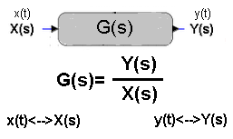
Fig. 15-1
Transmittance G(s) as a ratio of two transforms.
Chapter 15.2 Transmittance and differential equation on the example of the inertial term
The simplest but not trivial, because already described by the differential equation, is the inertial unit, e.g. with a time constant T=1 sec and K=1. We will examine the response to the unit step x(t)=1(t) and check whether it is consistent with the solution of the differential equation.
Fig. 15-2
This is a typical response of the inertial unit with K=1 and T=1 sec. For now, pay no attention to the equation in the time chart describing y(t). So far, the inertial unit G(s) is “something” from Fig. 15-2, which reacted to a unit step x(t)=1(t) with the time chart from Fig. 15-2.
You are also able to predict how other G(s) such as below will react to a unit step.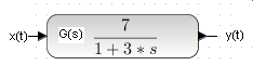
Fig. 15-3
In this way, having the transfer function G(s), you intuitively associate with x(t) and y(t), i.e. with time charts.
I am asking for a broader view.
There is a differential equation hidden in the transmittance G(s)!
Let’s go back to the tank with the hole for a moment Chapter 13.3.
Here, the output y(t) is related to the input x(t) differential equation x(t)=y'(t)+y(t) describing the filling of the tank with a hole. We will solve them using the operational calculus. We will subject both sides of this equation to the operator transformation s. We can do this because we know that each time function f(t) corresponds to its lovebird F(s). Vice versa too. We write it as f(t)<=>F(s).
That is
x(t)=y'(t)+y(t)
x(t)<=>X(s) here x(t)=1(t) (unit step)
y(t)<=>Y(s)
y'(t)<=>sY(s)
In the last transformation, we used a wonderful property of the operational calculus that the transformation of the derivative of f(t) is s*F(s).
If the operational calculus did not have this miracle, it would simply be useless.
Thus, the differential equation
x(t)=y'(t)+y(t)
transformed into an operator equation
X(s)=s*Y(s)+Y(s)
The last equation can be written as: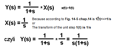
Fig. 15-4
We already know the Y(s) transform. All you need to do is find a wise book a second lovebird of the pair
y(t)<=>Y(s).
Where to start? Probably from Fig. 14-5 of chapter 14, where there is a piece of a wise book. There are only a few pairs there, but we’re lucky because we found the f(t)<–>F(s) pair we’re interested in.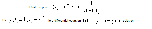
Fig. 15-5
Let me remind you that e=2.71828… is one of the most important numbers in mathematics. The output y(t) was calculated as solutions to the differential equation describing the transfer function G(s) from Fig. 15-2, i.e. pure theory.
Xcos in Fig. 15-2 did the same. So the line should coincide with the y(t) values.
Let’s check for e.g. t=0 sec, t=1 sec and t=7 sec.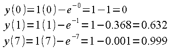
Fig. 15-6
That’s right!!!
Chapter 15.3 Transmittance and differential equation for any dynamic unit
We have already shown that for an object described by a simple differential equation
x(t)=y'(t)+y(t)
corresponds to the transmittance G(s) of the inertial unit with the parameters k=1 and T=1 sec.
The figure below shows how the transmittance is created with a more complicated differential equation e.g. of degree 3.
In an analogous way, the transmittance will be created based on a differential equation of any degree.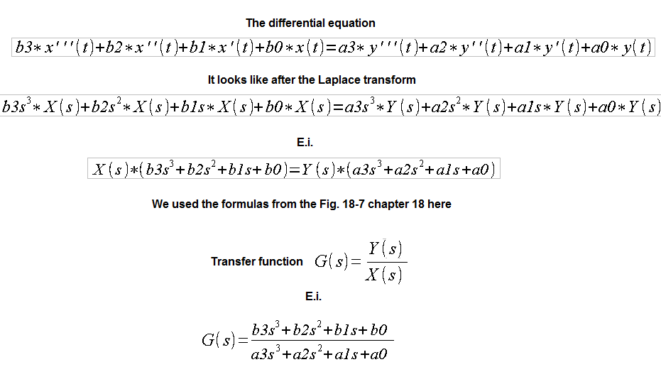
Fig. 15-7
So we see that the transfer function G(s) is a quotient where the numerator L(s) and the denominator M(s) are polynomials of the appropriate degrees. Usually L(s) has a lower degree than M(s) and most often it is only L(s)=bo, in addition bo=1 and the denominator is a product of polynomials of the first or second degree.
For example, the two-inertial unit has 2 first degree polynomials in the denominator
M(s)=(1+s*T1)*(1+s*T2)
Let’s check the response to the transfer function jump from Fig. 15-7 with specific parameters of the denominator M(s) and the numerator L(s).
M(s)–> a0,a1,a2,a3
L(s)–> b0,b1,b2,b3
Fig. 15-8
We can see how the higher derivatives mix in the time chart. Especially since the coefficients for these derivatives are small. What if they were big? Fear to think!
For most transmittances, the gain K in the steady state can be easily determined. It is simply the absolute term b0=1.25 in the transmittance numerator, when in ao=1 the denominator. If ao is different from 1, divide the numerator and denominator by ao.
Of course, this is the case when G(s) applies to stable systems. Not those in which any disturbance causes G(s) to become a generator. You know a lot about the transmittance response G(s) unit step 1(t).
Output y(t=2)=0, which is obvious.
And in steady state y(t)=bo=K.
And what happens in the transitional state (“between”), i.e. for t=2…15sec, corresponds to the other transmittance parameters at s.
These are the coefficients a1, a2, a3 and b1, b2, b3 the specific values of which are visible in the transmittance G(s) in Fig. 15-8.
Chapter 15.4 Resultant transmittance or combining transmittances
Blocks can be combined using the following method:
– serial
– parallel
– with feedback
Combinations of these methods are also possible.
Chapter 15.5 Serial connection of blocks
Fig. 15-9
It is a series connection of two inertial blocks G1(s) and G2(s).
You have an example at home. First, hot water (probably 70 ° C) is supplied to the radiator, which will heat up relatively quickly, then the radiator will heat the room, or more precisely, the place in the room where the thermometer is placed. The first time constant is small – a few minutes, the second is large – more minutes. A more accurate model would also take into account the To delay.
I don’t want the experiment to last an hour and a half. Therefore, our model has much smaller time constants T1=3 sec and T2=5 sec.
– The input signal is the step x(t)=1(t)
– intermediate y1(t) typical inertia
– output y(t) typical two-inertial with a characteristic point of inflection.
Especially since:
– taking into account the “heaviness” of 2 series-connected inertial units in the transition state, it should be y1(t)>y(t)
– in steady state y(t)=y1(t)=x(t)
This is confirmed by the time charts.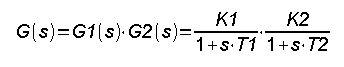
Fig. 15-10
The resultant transmittance G(s) of blocks connected in series is the product of their transmittance G1(s) and G1(s). This formula is most obvious for proportional units, eg amplifiers, whose gain is the product of the gains K=K1*K2. In Fig. 15-9, there were 2 inertial transmittances with the parameters K1=1, T1=3 sec and K2=1, T2=5 sec.
Chapter 15.6 Parallel connection of blocks
Fig. 15-11
In parallel connection, the input signal x(t) “spreads” from one tap node to 2 inputs of inertial units. Then the outputs of these units y1(t) and y2(t) add up in the summation node. It is clear from the time charts that the output is the sum of the outputs of the two units, which means that the resultant transmittance is the sum of the individual transmittances.
A side note.
The time chart y(t) looks like a typical inertial unit. However, try adding 2 fractions G(s)=G1(s)+G2(s). There will be no inertial or even two-inertial unit. There will be some s in the numerator L(s) of the resultant transmittance G(s).
Remember!
There is always in parallel connectiona a spread node at the input and a summation node at the output! If there was also a spread node on the output, it would be as if you connected the parallel outputs of 2 different voltages.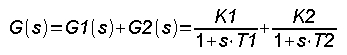
Fig. 15-12
The resultant transmittance G(s) is the sum of G1(s) and G2(s). In our case, there were 2 inertial transmittances with the parameters K1=0.5, T1=3 sec and K2=0.5, T2=5 sec. For proportional units, e.g. amplifiers, the transmittance or gain is also the sum of the reinforcements K=K1+K2.
Chap. 15.7 Negative Feedback Connection
Series and parallel connection is easy to understand. It is different with negative feedback. It is not known what is cause and what is effect. Virtually all automatics is negative feedback in one form or another. For now, let’s treat feedback dispassionately-purely mathematically with the help of operational calculus. Given the transmittance of the open system G(s) let us calculate the transmittance of the closed system Gz(s).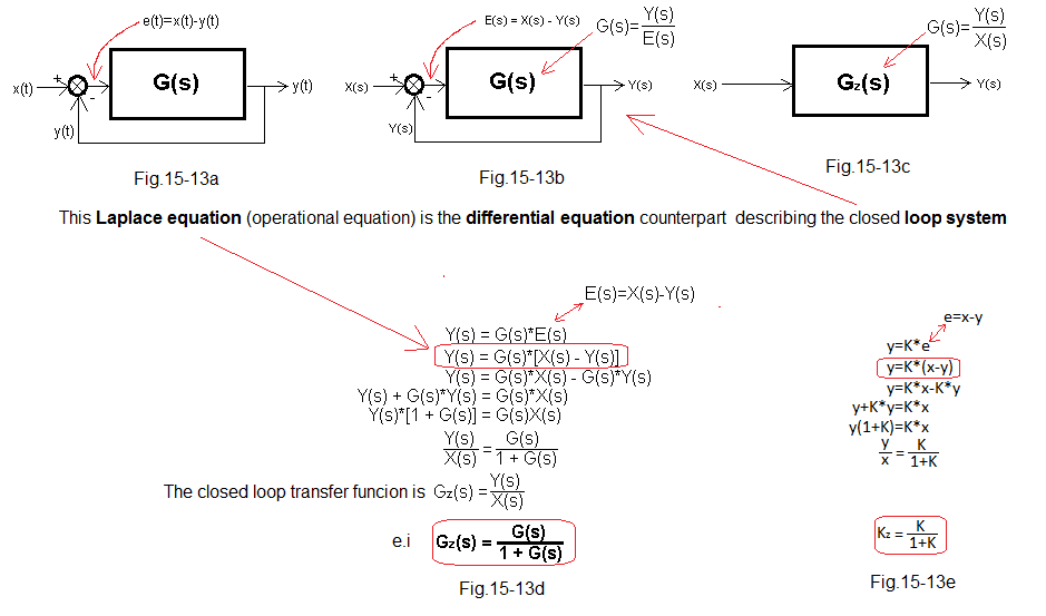
Fig. 15-13
Negative feedback was created after introducing the signal difference e(t)=x(t)-y(t) to the input of the open system G(s). The output signal y(t) was reintroduced (returned!) to the input G(s) with a negative sign as shown in Fig. 15-13a. Hence the name – Negative Feedback System.
People have long noticed that such a structure has a lot of advantages. For example, the output signal y(t) tries to imitate the input signal x(t) regardless of interference. The second benefit is the ability to speed up the operation of the system.
Fig. 15-13a shows the transmittance signal paths of transmittance G(s), which is closed with a negative feedback loop.
Fig. 15-13b was created by transforming the time signals in 15-13a to the appropriate Laplace transforms.
Fig. 15-13c The transmittance of each system is the ratio Y(s)/X(s). Therefore, the transmittance of a closed system is Gz(s).
Fig. 15-13d Derivation of the formula for the transmittance of a closed system Gz(s).
Fig. 15-13e Derivation of the formula for the amplification of a closed system Kz in steady state. This formula is easiest to derive as Kz=Gz(0), i.e. by substituting s=0 to the formula Fig. 15-13d. But we went a different way. We started with a very important observation that in steady state y(t)=K*e(t). For many this is obvious, but on the other hand this principle is so important that I will try to justify it in the next chapter. Since in the steady state the signals are constant->x(t)=x and y(t)=y, we can easily get to the formula for Kz. Let’s also check whether the derived formula for Gz(s) is true for any specific transmittance G(s).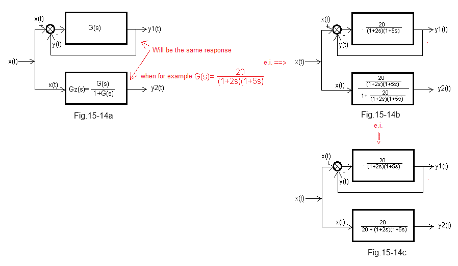
Fig. 15-14
The specific transmittance G(s) is a two-inertial unit with the parameters K=20, T1=2 sec, T2=5 sec.
The upper one in Fig. 15-14a is the G(s) covered by negative feedback, and the lower one in Fig. 15-14a is the equivalent transmittance Gz(s) of the upper one in accordance with the derived formula in Fig. 15-13.
Fig. 15-14b is the implementation of 15-14a for our specific transmittance, and Fig. 15-14c is the same after elementary transformations.
The inputs of the upper and lower blocks receive the same unit step x(t), so we expect the same answers y1(t)=y2(t).
Will it be?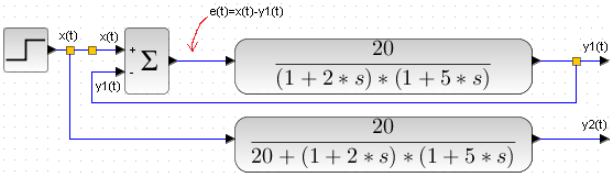
Rys. 15-15
The diagram corresponds to Fig. 15-14c.
Fig. 15-16
The negative feedback system and its equivalent transmittance give the same response to x(t).
Note the gain Kz in the steady state. Does it not resemble the formula for the transmittance of the equivalent system Gz(s)? In addition, the y(t) signal in steady state is almost equal to the x(t) signal! So the output signal y(t) tries to imitate the input signal x(t). Just like an employee tries to follow the orders of the manager.
It was just a fairly dry and mathematical introduction to feedback.
Therefore, the whole of the next Chapter 16 is only about this topic..
Chapter 15.5 Conclusions
1. The transmittance G(s) is the equivalent of a differential equation describing a given dynamic object
2. From the parameters G(s) we can easily determine the gain K in steady state -> Fig. 15-8
3. In Fig. 15-7 and Fig. 15-8 transmittances G(s) were given as “naked” quotients where the numerator and denominator were the classical form of the polynomial. They are often given in a slightly modified form, such as

Fig. 15-17
The case is simple. Here you can see at first glance that we are dealing with a two-inertial unit with parameters k,T1,T2–>Fig.15-17a or with an oscillating element with parameters k,T,q–>Fig.15-17b. This would not be visible in the “naked” quotient Fig. 15-17c
4. Transmittances of connected blocks:
– in series
-in parallel
– with negative feedback
can be replaced by a single equivalent transfer function