Operational Calculus
Chapter 14 Operational Calculus
Chapter 14.1 Introduction
Each time function f(t) is assigned its Laplace transform F(s)
which is most often the quotient of 2 polynomials of the complex variable s.*
f(t) ==>F(s) (Fig. 14-1a)
And vice versa Each Laplace transform F(s) is assigned a time function f(t)
F(s) ==>f(t) (Fig. 14-1b)
Ultimately, “it works both ways”
f(t)<==>F(s) (Fig. 14-1c)
*If you don’t know complex numbers, don’t worry. Treat them like regular s variables. Below is an example where f(t) is a function of time and F(s) is a fraction. In it, the numerator L(s) is a polynomial of degree 2 and the denominator of degree 3: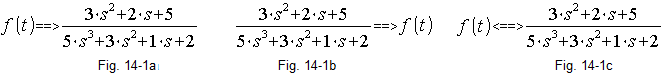
Fig. 14-1
Relations between f(t) and F(s)
An even more concrete example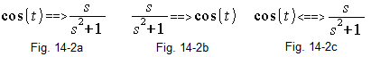
Fig. 14-2
Example for the function f(t)=cos(t)
Note 1
In fact, f(t)=cos(t) only for t>=0. For t<0 f(t) =0!!! The rule applies to all functions f(t) listed below. This is due to the fact that in automatics everything starts at a specific time, most often for t=0. For example, the function unit step x(t)=1 for negative t is zero.
Note 2:
The expression f(t)=F(s) would be absolutely pointless!
Chap. 14.2 Relationship between F(s) and f(t)
The time function f(t) and its transform F(s) are related by the equation
Fig. 14-3
Formula for F(s) for function f(t)
For simple functions f(t) it can still be calculated. For more complicated ones, too, but only once to pass the student exams. I even thought about giving this formula. Especially since, apart from the concept of integral, the number s is an obstacle. There is the so-called a complex number, and to make it even more fun in the exponential function.
If it bothers you, then you can let it go. Then treat the Laplace transform as an ordinary assignment
f(t)<=>F(s). As if there was a very clever book somewhere, and there were pairs f(t)<=>F(s). Even an automatics theorist sometimes uses such a book. Its piece, i.e. only one pair for f(t)=cos(t) is Fig. 14-2c. More pairs are Fig. 14-5. As for the complex number s, treat it like a good real number. Just be aware that it isn’t.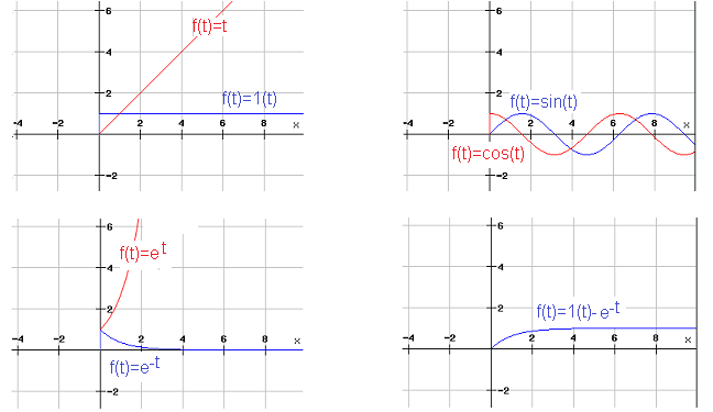
Fig. 14-4
Functions f(t) for which appropriate transforms F(s) are assigned in Fig. 14-5.
The time charts are there to emphasize that all f(t) functions have a zero value for t<0. It is generally the case in automation that something starts at t=0, e.g. unit step f(t)=1(t).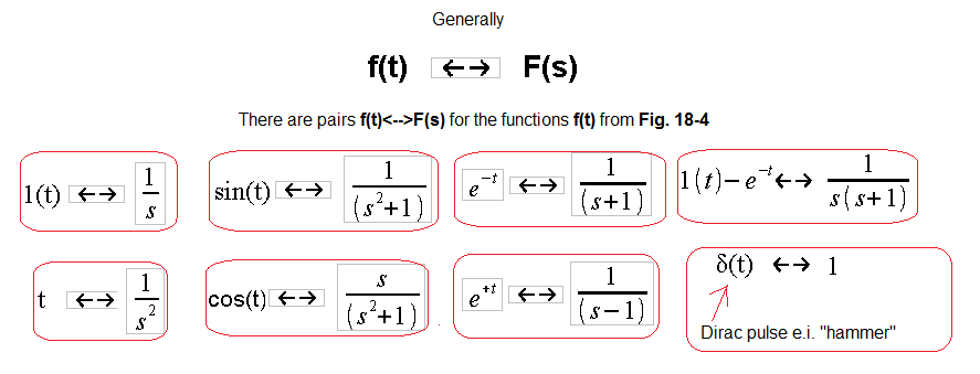
Fig. 14-5
The figure also shows the pair δ(t)<==>1, i.e. the Dirac impulse and its transform F(s)=1.
The number e=2.7182… in 3 formulas is one of the “most famous” in mathematics next to 0, 1, PI…
Chapter 14.3 How does differentiating f(t) affect its transform F(s)?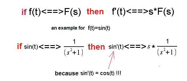
Fig. 14-6
This is the most important theorem of the Operatotional Calculus. Without it, there would be no Operatotional Calculus!
Note
In fact, the formula for the derivative transform is a little different, but it can be used in most cases. And so be it. After all, this course is just an introduction to automatics.
The formula can be easily generalized to further derivatives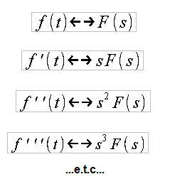
Fig. 14-7
Calculating the derivative of a function requires some effort. However, calculating the transform of the nth derivative is a piece of cake. Just multiply F(s) by the nth power of s. This rule makes it easy to solve linear differential equations. You will find out in the next chapter.