Automatics
Chapter 16 How does feedback work?
Chapter 16.1 Introduction
Feedback consists in the fact that the output signal y(t) returns back to the input.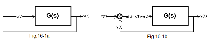
Fig.16-1
Fig. 16-1a
The y(t) signal from the output returns directly to the input. But what is the cause and what is the effect? Did the egg come first or the chicken? Not to mention more existential questions. So let’s treat the scheme as a curiosity.
Fig.16-1b
So you need some contact with the outside world. It is implemented as a calculation of the control error i.e. e(t)=x(t)-y(t) in the so-called subtractor node. This is the most important scheme in automatics because y(t) tries to imitate x(t). It must be as obvious and instinctive to you as riding a bike! Understanding the mechanism of this imitation is the main goal of this chapter.
Chapter 16.2 How does positive feedback work?
Chapter 16.2.1 Introduction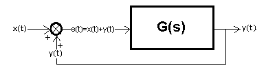
Fig. 16-2
Positive feedback.
That is, in which the sum of signals e(t)=x(t)+y(t) is fed to the input, instead of the difference as
in Fig. 16-1b. Rather, it is something harmful. Accident at work. For example, when the fitter gets the cables wrong, and instead of the “-” input of the controller, he will go to the “+” input. It is easier to understand than negative feedback, and that is why we are analyzing this case.
Chapter 16.2.2 Positive Feedback “Large”
Why “big”? You’ll find out when “small” is mentioned.
This is the version of Fig. 16-2 when G(s) is the inertial unit with the parameters K=1.5, T=3 sec. The signal from the output returns to the input and is added to the input Dirac signal x(t) – “pins” or in other words “flick”. Note that K=1.5>1!
Fig. 16-3
The sum of the signals s(t)=x(t)+y(t) enters the input of the inertial unit. Initially, x(t)=y(t)=0. So s(t)=0+0=0 and nothing happens. But in the fifth second, a Dirac=”pin” appears. This signal will pass through the inertial unit as a “damped pin” with a lower amplitude and increased by 1.5 times. At first, this “repressed pin” is so small that it cannot be seen on the time chart, but it will immediately return to the input and again be increased by 1.5 times. It will come back again and will be increased by 1.5 times…etc. Classic avalanche effect. The system was unstable from the beginning, although it was not visible until the fifth second. But all it took was a small touch for a disaster to ensue.
In automatics, positive feedbacks are avoided. However, in social life, economy … it will not always work out. A common example is the stock market. The company appears to be stable. All it takes is a rumor (the equivalent of a “pin”) that its stock will start to rise. As they grow, people buy –> the more they grow –> the more they buy…etc.
Returning to our example, we could make such a hypothesis. A system with positive feedback is always unstable. Any unbalance of it causes the signal to grow to +/- infinity. Is it always like this? Let’s check the next example.
Chapter 16.2.3 Positive feedback “Small”
Why “small”? Previously, the transmittance counter was 1.5>1. And when the numerator is less than 1, e.g. 0.8? Check it out. I will anticipate the facts. Despite the positive feedback, the system will be stable. Therefore, we can afford a step-type input x(t).
Fig. 16-4
Here the numerator of the transmittance G(s) is 0.8. Or in other words – steady-state gain of an open system (i.e. before closing the feedback loop) K=0.8 and T=3sec. The response of a closed system resembles an inertial unit. And so it is! In this case, let us determine the gain Kz of this system from the time chart and its time constant Tz see–> Fig. 3-4 Chapter 3.
The result Kz=4 and Tz=15 sec tells us that positive feedback increases:
– amplification from K=0.8 to Kz=4
– time constant from T=3 sec to Tz=15 sec – read more inertia
A long time ago, when there was no electronics yet, only radio engineering, and lamps or transistors were very expensive, positive feedback was used to increase the gain. Unfortunately, at the expense of greater inertia, i.e. at the cost of limiting the frequency response. In the next section, we will prove that it is indeed an inertial unit. Now we only assume that it is. And the conclusion is that a positive feedback system can be stable!
Chap. 16.2.4 Transmittance Gz(s) of a positive feedback system
Derive the formula for Gz(s) for a system with positive feedback.
Fig. 15-13, chapter 15 will be helpful in this. Instead of E(s)=X(s)-Y(S) put E(s)=X(s)+Y(s).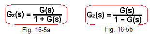
Fig. 16-5
For comparison purposes, Gz(s) of the system with negative feedback are shown -> Fig. 16-5a.
If you managed to derive the formula for positive feedback, you will get–> Fig. 16-5b.
Let’s check this formula, e.g. for the transmittance in Fig. 16-3 and Fig. 16-4
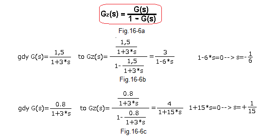
Fig. 16-6
Fig. 16-6a – transmittance of the system with positive feedback
Fig. 16-6b – an example when K=1.5>1, as in Fig. 16-3. The system is unstable. The root of the denominator is positive.
Fig. 16-6c – example when K=0.8<1, as in Fig. 16-4. The system is stable. The root of the denominator is negative.
Here the denominator was a polynomial of degree n=1. Our observation can be generalized to any polynomial of degree n.
By the way, we learned one of the basic theorems of automatics.
The system is stable if the transmittance denominator contains only negative roots.
More precisely, for those who know the so-called complex numbers.
They will be discussed in Chapter. 19.
The system is stable if the transmittance denominator contains only roots with a negative real part.
So we will replace the word negative root with the word negative real part of the root.
Chap. 16.2.5 Positive Feedback Conclusions
1- We rather try to avoid it
2- Usually, but not always, positive feedback is the cause of instability.
3- General remark regarding any transmittances.
The positive root of the denominator of the transmittance G(s) is instability!
Chap. 16.3 How does negative feedback work?
Chap. 16.3.1 Introduction
In automatics, negative feedback is used, the most important feature of which is that the output signal y(t) “tries” to imitate the input signal x(t). That’s why the rockets hit the target, because they track something there, the furnace tries to maintain the temperature of the liquid +75ºC when the set value x(t) is also +75ºC, etc…
Chap. 16.3.2 How does the inertial unit in an open system come to a steady state?
Before we consider how the negative-feedback inertial unit comes to steady state, let’s answer the easier question above.
Fig. 16-7
Inertial unit in an open system.
We are observing signals:
– input signal-step x(t)=1(t)
– output signal y(t) of the inertial unit K=5 and T=3sec
– goal K*x(t) (K=5)<– What is a goal? You’ll know in a moment.
The steady state y=K*x(t)=5 is the goal y(t) is aiming at. The “driving force” that causes y(t) to increase is the difference–the vertical green bar U=K*x(t)-y(t). At the beginning of the step x(t) in 1 sec the signal y(t)=0. Therefore, the “driving force” – the vertical green bar is the greatest here and y(t) starts at maximum speed. Then U gradually decreases (e.g. in 5 s U≈1.3) and the growth rate also decreases. After 25 s, the driving force U has dropped to zero. The goal was achieved y(t)=K*x(t).
The most important conclusion
Output y(t) tends to equilibrium
y(t)=K*x(t)
in which the “driving force U” disappears – a vertical green line
The conclusion is so obvious that the reader wonders what the author means? And this is just an introduction to the next chapter.
Chap. 16.3.3 How an inertial unit with negative feedback comes to a steady state.
Fig. 16-8
Inertial unit with negative feedback.
The signals are:
– output y(t)
– goal K*e(t) (K=5)
Here y(t) also pursues the goal K*e(t), which, however, unlike the open system, is time-varying. The “driving force” that tries to bring the goal K*e(t) and y(t) together is also the difference U=K*e(t)-y(t) in the form of a vertical green line. The more the difference U – “driving force” is greater, the stronger the goal lines K*e(t) and y(t) “stick” to each other.
The output y(t) tends to the state of equilibrium y(t)=K*e(t) in which the “driving force U” disappears – the vertical green line
And when will y(t) stop growing? Or in other words, when will it be steady state. Then, when the goal is achieved, when the driving force (vertical green U line) disappears! That is, when y(t)=K*e(t).
This is the case not only for the inertial unit, but for each dynamic units with negative feedback, which has a gain K in steady state. The experiment confirms something very important in automatics.
Just like a pendulum out of balance, it will return to its steady state, which is the lowest position
Thus, a stable system with negative feedback will return to the state y(t)=K*e(t).
This only applies to stable systems. And that won’t always work.
Do you remember Fig. 15-13e in Chapter 15? In it, you weren’t completely convinced yet that steady state with negative feedback is y=K*e. Now you know that this is the case and the proof of this is the time charts 5*e(t) and y(t) that met at y(t)=5*e(t).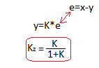
Fig. 16-9
The lower formula for the Kz gain of a closed system results directly from y(t)=K*e(t).
Also y=0.83 in Fig. 16-8 confirms our calculations.
Rozdz. 16.3.4 How does an inertial unit with large negative feedback come to a steady state?
We will also add the observation of the control error e(t)=x(t)-y(t)
Fig. 16-10
The oscilloscope settings are such that you can see the entire “variable target” 100*e(t) where e(t)=x(t)-y(t). The very large initial 100*e(t) compared to the signals x(t),y(t) and e(t) are conspicuous. This is the main conclusion of this experiment. Later you will learn that it is a P-type control system, in which s(t)=100*e(t) is the control signal. The “pin” 100*e(t) at the beginning of the stroke is characteristic here.
On the one hand, a good “pin” causes almost instantaneous arrival to a steady state compared to an open system. This causes a technical problem. If it was a steady-state furnace, e.g. 10kW, the “pin” wants 100 times more – > 1MW! We’ll come back to the topic.
With these oscilloscope settings, there is a very inaccurate view of what is most important, i.e. the y(t), x(t) and e(t) signals. It can be roughly seen that in steady state there is almost x(t)=y(t)=1 and e(t)=0. So let’s change the settings of the oscilloscope to see these signals.
You will get a time chart exactly the same as Fig. 16-11. The difference is only in what you can’t see – in the oscilloscope settings.
Fig. 16-11
You see the same time chart, only in the range y=0…1.2 and not y=1…100 as before. Although the “pin” has been cut off, the remaining signals – x(t), y(t) and e(t) are clearly visible. Thanks to the strong feedback (the y(t) signal returns 100 times stronger!) and y(t) almost immediately it reaches a steady state y(t)=0.99. This is a confirmation of the steady-state Kz amplification formula from Fig. 16-9.
Chap. 16.3.5 How does a two-inertial unit with negative feedback come to a steady state?
The previous inertial unit was coming to a steady state “from below”. i.e. y(t) was always smaller than 5*e(t). However, it is known that control systems often do this with oscillations. An example will be the two-inertial unit with feedback.
Fig. 16-12
The signal y(t) reached the value in which y(t)=K*e(t) in just 6 seconds. It seems to be an equilibrium state, but y(t) keeps increasing. Why is it like that?
– First, it is not in equilibrium, because y(t) is “moving”. It is true that y(t)=K*e(t) but the derivatives of y(t) (e.g. velocity y(t)) are not zero!
– Secondly, this is a two-inertial unit. The y(t) signal can increase for a while when the input signal is zero or even negative!
Go back to Fig. 16-8, that is to inertial unit, for a moment. Here K*e(t) is always greater than y(t). Or in other words y(t) arrives at K*e(t) from below. Because the “driving force” U – the vertical green line was positive all the time.
And what about Fig. 16-12?
Here, up to 6 seconds, the “driving force” in the form of a green line is positive. Further, the accumulated energy of the two-inertial term makes it exceed the apparent equilibrium state y(t)=K*e(t) and the “driving force” becomes negative. So the “driving force” becomes the “braking force”. The braking effect is clearly visible. Red y(t) decreases the growth rate until it becomes negative. Now y(t) “turns around” again and after a few oscillations it reaches a real (and not “fake” as in 6 sec) equilibrium state, in which y(t)=5*e(t)=0.83 .
Chapter 16.3.6 Static and astatic units
Let me remind you that for G(s) steady-state gain K we can calculate 2 methods:
1- From the time charts–>K=y(t)/x(t) in steady state, e.g. in Fig.16-12
2- Directly from the transmittance by calculating K=G(s=0) as below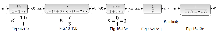
Fig. 16-13
Fig. 16-13a inertial unit – no comment
Fig. 16-13b two-inertial unit – no comment
Fig. 16-13c the real differentiating unit. In steady state y(t)=0!
The above gains K in the steady state are probably obvious. Maybe a small question mark is Fig. 16-13c but it will pass somehow.
These were the so-called static units which give a specific finite response in a steady state per unit step x(t)=1(t). However, the problem arises with the ideal integrating unit in Fig. 16-13d, where we have to break the holy rule “Remember, damn, never divide by zero“. However, if we break it, i.e., divide it by a number infinitely close to 0, we get K=infinity. This unit and others (e.g. Fig. 16-13e) that have at least one zero root in the denominator are astatic units.
Fig. 16-13d integrating unit
Fig. 16-13e the real integrating unit, i.e. with inertia
And what are steady states for the astatic units?
Chapter 16.3.7 Going to a steady state of the astatic unit in an open system
The title is provocative. You’ll find out why in a moment.
In order to show the typical features of the integrating unit as astatic, the input will be given a signal x(t) which:
– At the beginning it is a positive unit step
– then it is 0
– then it is a negative unit step
– ends as 0
Fig. 16-14
It can be, for example, an ideal DC motor. Ideal, because it does not take into account the mechanical (mainly rotor mass) and electrical (winding inductance) inertia. The output signal y(t) is the position as positive or negative angle of rotation. The input signal is the supply voltage x(t) which changes in 4 stages:
stage 0…3 sec voltage x(t)=0V–-> the motor is stationary, i.e. y(t)=0—>0V
stage 3…10 sec. voltage x(t)=+1V the motor turns right
at a constant speed–-> y(t) increases linearly –>0…+7V.
stage 10…30 sec voltage x(t)=0V–> the motor is stationary,
i.e. at the level y(t)=7–>+7V
stage 30…40 sec, the voltage x(t)=-1V, the motor turns left
at a constant speed–-> y(t) decreases linearly–>+7V…-3V.
stage 40…60 sec voltage x(t)=0V –> the motor is stationary, i.e. y(t)=-3–>-3V
Conclusions
1- The output signal y(t) increases at a constant rate when the input signal x(t) is constant positive
2- The output signal y(t) decreases at a constant rate when the input signal x(t) is constantly negative
3- The rate of rise or fall is proportional to the input signal x(t)
4- Output signal y(t) will stop when input signal x(t)=0.
Now you know why the title was provocative. With a unit step y(t) will never reach a steady state, i.e. one in which it is stationary. More precisely, in the steady state y(t) is infinity, i.e. the gain K is formally infinity.
Chapter 16.3.8 How does the negative feedback integral unit come to a steady state?
The integral unit is an example of an astatic unit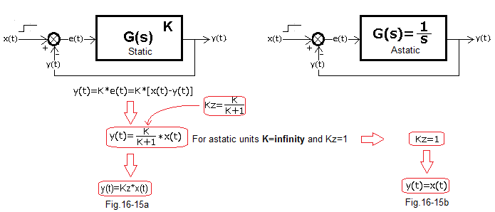
Fig. 16-15
Fig. 16-15a is a tirelessly repeated formula for gain Kz of a closed system for static units.
Fig. 16-15b are analogous formulas for astatic units. They strike with their simplicity and this is due to the fact that for astatic gain K=infinity.
In steady state y(t)=x(t). So the output y(t) ideally reproduces the input x(t). That is, it provides zero control error e(t). This is the goal of every automatics engineer. So says the theory. What about intuition?
Fig.16-16
You can see how the integrating unit comes to a steady state y(t)=x(t)=1. Compare with Fig. 16-8 with the inertial unit which is static. In it, the “driving force” u=5*e(t)-y(t) that strives for the state of equilibrium defined by the formula in Fig. 16-8 was y=0.83 when u=5*e(t)-y(t)=0.
Here, however, the driving force is the error e(t). Simplicity is beautiful!
When x(t)>y(t) (or e(t)>0) then y(t) increases as in any decent integrating unit. I will add that it is growing at a slower and slower speed because e(t) is constantly decreasing. In a steady state, this speed is, of course, zero. That is e(t)=0 and y(t)=x(t)=1.
Let’s check how a slightly more complicated astaticunit, i.e. integrating with inertia, comes to equilibrium.
Chapter 16.3.9 How does the integral unit with inertia and negative feedback come to a steady state?
As in the previous point, we studied the ideal integral unit in the feedback, so now we will consider the real integral unit. It will still be a DC motor, but taking into account the electromechanical inertia. This time we will not study open system. It will give similar results as in Fig. 16-14, only the time charts will be smoother, as in Fig. 8-5, chapter 8.
Fig. 16-17
You can see how positive e(t) (like a green line) drives y(t) towards equilibrium, and negative e(t) slows it down. Note that although, for example, in 6 sec. there is a state x(t)=y(t)=1 but only temporary. The motor has a certain energy that “makes” it continue to spin above the steady state x(t)=y(t)=1. Then a negative e(t) makes him brake. Eventually, after several oscillations, the steady state x(t)=y(t)=1 will occur. So e(t)=0.
Chapter 16.4 Conclusions
Chap. 16.4.1 Transmittances of a closed system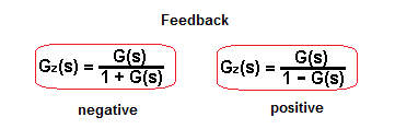
Fig. 16-18
The formulas apply to all G(s) – static and astatic units
Chapter 16.4.2 Static systems with negative feedback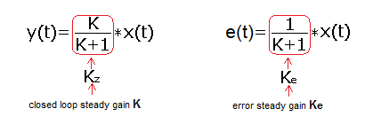
Fig. 16-19
In automatics, y(t) to tries to imitate x(t). This is true (“almost”) when the open-loop gain K is large. Then it is “almost” Kz=1 Ke=0.
Chapter 16.4.3 Astatic systems with negative feedback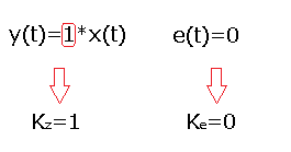
Fig. 16-20
The gain Kz is equal to 1 and the error Ke equals 0. It follows that astatic systems provide zero fixed error e(t).
That is in steady state y(t)=x(t). They are easier to understand than static ones. Later you will learn that the zero control error e(t) is provided by the integral component I of the PID controller.
Chapter 16.4.4 What was not in this chapter
1- Instability in negative feedback –> We will deal with this topic in the next chapter.
2- In a static, e.g. inertial, open system when K=1, the steady state provides y(t)=x(t). Then why complicate life with some feedback? The answer is simple
Negative feedback provides:
– resistance to external disturbances
– improves the dynamics, i.e. the speed of reaction.