Automatics
Chapter 1 Introduction
Introduction Chapter 1
If you want to know how a regulator works, including the king of regulators – PID, then this course is for you! Especially if you don’t feel confident in the world of integrals and derivatives. You will independently explore various objects in real time! It is important that the waveforms will be of “normal” duration – usually in the range of 10 … 120 sec. You can see everything moving and crawling! Not so when the waveform lasts only 30 µs, or vice versa 30 years. It is also completely different than time charts in books, e.g. regarding the inertial unit. That is, to put it simply, observing the increase in the temperature of the furnace when I give the heater abruptly (“suddenly”) 230V voltage. You’ll notice that the rate of temperature increase (not the temperature itself!) is greatest at the beginning, then gradually decreases. Eventually, the temperature will stop at, for example, 300°C. When I repeat the experiment with half the previous power, the course will be similar, but instead of 300°C it will be 150°C.
The inertial element as a furnace model is very simplified. The time chart of a real furnace will be slightly different. For example, the initial rate of temperature increase is zero. Also at half the power will be, for example, +170°C. and not +150°C But that’s a completely different story…
There is very little in the course for “word of honor”. We try to check everything.
For example. We check according to the Hurwitz criterion whether a given object G(s) is stable, and then by touching the input with an impulse x(t), we try to throw it off balance. Learning consists in developing individual schemes of Control Systems and examining their properties.
The further into the forest, the more trees there are. We start by examining the simplest dynamic units –> Chap. 2…10 and we end up with more interesting topics such as Cascade Control, Closed-Open System, Ratio Regulation…
Your job is just to study the influence of various parameters on the time charts and draw appropriate conclusions. You will feel like a dispatcher in the Refinery Control Room , watching the technological process on monitors.
Nay. You can do forbidden things! For example, drill a hole in the column through which the distillate escapes. This example is one of the basic concepts of so-called automation disturbance. The control system will compensate for the disturbance (escaping distillate) with an additional inflow. You can also change the settings of the PID controller so that the oscillations do not go out. In this way, you safely gain experience, like a pilot practicing dangerous situations on a Jumbojet simulator.
I emphasize. These will not be ordinary “static” drawings, e.g. response to a unit step of an inertial unit, but a real cinema with mp4 files! I performed all the experiments in the SCILAB program, more precisely in its main application Xcos. Then I recorded their waveforms using the video program Active Presenter (“cinema”). So you don’t have to go into SCILAB, just press the start video button. I guarantee you that you will feel the dynamics of the process better than on ordinary charts.
Note!
If you’ve had little to do with automatics so far, the rest of this chapter, which summarizes the entire course, may be a bit intimidating. Then don’t worry. Read it to the end and move on to Chapter. 2 Proportional term.
Basic Dynamic Units → Chapters. 2…10
Each chapter is an examination of a separate dynamic unit, from the simplest to the more complex. It consists in providing the appropriate input signal x(t) and observing the output signal y(t).
The source of the input signal x(t) can be:
– Unit step function generator – most often
– Ramp signal generator
– Virtual potentiometer slider
– Dirac impulse, i.e. a “short tap of the input with a hammer”
The output signal y(t) can be observed by:
-an oscilloscope, i.e. your monitor – most often
-digital virtual meter
-bar graph, i.e. an analog virtual meter in the form of a black vertical line
You will associate the transmittance parameters G(s) with the response y(t) to the input x(t). The most common is a single step.
Animation example
Fig. 1-1
Oscillatory Unit when the input is a unit step function
To start the animation, click on the video triangle.
The parameter K=2 and T=2sec can be read from the time chart
After reading chapters 2…10, you can easily predict, for example, the behavior of 2 similar-looking dynamic members in Fig. 1-2.
No Higher Math!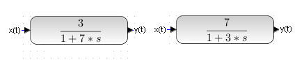
Fig 1-2
A bit of maths → Chapters. 11…14
If you are familiar with the topic, skip to Chapter 15.
I tried to make the course useful also for people who are not familiar with higher math.
Therefore, it contains several chapters on derivatives, integrals, simple differential equations and operational calculus. Because how can you not understand integration and differentiation when you have:
– differentiator which differentiates the input signal,
– integrator that integrates the input signal
Chapter 11 Differentiation
If you have a problem with the derivative, you will be enlightened by examining the differentiator.
Fig.1-3
The input signal is the parabola x(t)=t².
It is differentiated twice by the differentiator. The experiment shows that the first derivative of x'(t)=2t and the second derivative of x”(t)=2. It agrees with the theory.
Chapter. 12 Integration
Why exactly a unit step x(t)=1(t)? Because it is difficult to find a simpler function and it is easy to calculate the integral denoted as the field S from it. Let’s treat the definite integral as the output y(t) of the integrating unit whose input is x(t)=1(t). It turns out that y(t)=t(t).
Note:
t(t) this is a function y(t)=0 for t<0
y(t)=t for t>0
Fig.1-4
Also, the integral as the area under the function will become obvious after examining the integrating unit. The area under the function x(t)=1 is y(t)=t(t). And that’s nothing but the integral of x(t)=1(t).
Chapter 13 Differential Equations
You didn’t know it then. But you have already dealt with differential equations in primary school by solving a problem like “a train goes from city a to city b with speed v“… After all, speed is a derivative of the distance, so…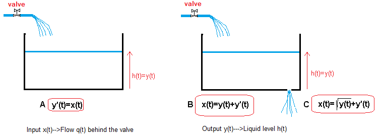
Fig.1-5
We will learn differential equations on the basis of less trivial examples:
A – differential equation of filling the tank without a hole.
B – simplified differential equation of filling a tank with a hole.
C – exact differential equation of filling a tank with a hole.
I will show animations as solutions to the above differential equations.
Chapter. 14 Operational Calculus
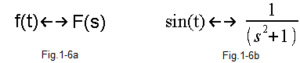
Fig.1-6
Each time function f(t) can be assigned a transform F(s) and vice versa–>Fig. 1-6a. The parameter s is the so-called a complex number. If you don’t know complex numbers, treat them temporarily as real numbers. In other words – don’t worry.
Fig. 1-6b is a version of Fig. 1-6a for the specific function f(t)=sin(t).
How is the transform F(s) derived from f(t)?
Never mind! Suppose there is such a smart book with all possible pairs f(t)<–>F(s).
The Operational Calculus has one nice feature. He would be worthless without her. It is easy to calculate the transform from the derivative of the f(t) function, i.e. the transform from f'(t). Simply multiplying F(s) by s like this:
How is the transform F(s) derived from f'(t)?![]()
Fig.1-7
This makes it easier to solve linear differential equations*. They are converted into ordinary algebraic equations in which polynomials of the nth degree of the variable s occur. And from them it is already possible to draw conclusions about automatic control systems.
What are the waveforms, what is the steady state output, what is the stability? e.t.c..
*Linear differential equations are an approximation to most control systems. Examples of these are differential equations A and B in Fig.1-5. Equation C, however, is not
CONTROL IN GENERAL → Chap. 15…22
Chap. 15 More about transmittance and connecting blocks
You will learn that:
The transmittance G(s) is equivalent to the differential equation describing a given dynamic object from the parameters G(s) we can easily determine the steady-state gain K
Connected block transmittances:
– in series
– in parallel
– with negative feedback,
can be replaced by a single equivalent transmittance Gz(s).
Chap. 16 How does feedback work?
You read the manual of a washing machine, cell phone or something else and you have problems. Although the guy writes wisely and in beautiful language, but something is missing. Exactly. The person writing the instructions is deep in the subject, because that’s all he does. For him, the operation of the device is as obvious as the operation of a flail. He simply does not want to offend the User with an exact translation of how it works.
The same is true with negative feedback. After all, all this follows from the formula shown below Fig. 1-8c! It concerns the transmittance Gz(s) of a system with negative feedback. In addition, this formula is very easy to derive. But how does negative feedback really work? The same y(t) signal at the output and input? A snake eating its own tail? Why the output signal y(t) “tries” to imitate the input signal, so called set value x(t)?
A good understanding of this problem is understanding the essence of automation. Without it, various Nyquists, Hurwitzes, state spaces… are worth nothing.
So let’s move on to the principle of operation of the flail.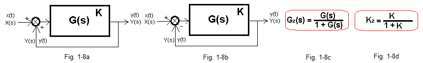
Fig.1-8
The chapter begins with the positive feedback in Fig. 1-8a, which is easy to understand. You will learn that not always a system with positive feedback is unstable. It becomes it only with higher K* amplification.
You will understand why in the negative feedback circuit in Fig. 1-8b, the y(t) output “tries” to follow the x(t) input. The most important thing is to understand the principle that the system tends to a steady state in which:
y(t)=K*e(t)
Like a pendulum that tends to its lowest point. You will see that the values of K*e(t) and y(t) are attracted to each other. At the beginning of the x(t) jump, the difference between K*e(t) and y(t) is large, then it decreases until the equilibrium state where y(t)=K*e(t)!
If the “clinging” waveforms K*e(t) and y(t) are obvious to you, then you are feeling negative feedback! From the equilibrium state y(t)=K*e(t) follows the formula for the gain Kz of a closed system in steady state Fig.1-8d. It is, moreover, a special case of the transmittance Gz(s) of the closed system in Fig. 1-8c.
The y(t) does not always end with a state of equilibrium, but with undying vibrations. The system is unstable. Then the formula for Kz makes little sense, but not entirely. Namely, the oscillations have a constant component c=Kz*x(t) where x(t) is a unit step.
*K is the gain of the object G(s) in steady state.
Chap. 17. Instability, or how oscillations are created?
We will conclude that the cause of the instability is the delay between the input and output signal. The easiest way to see this is to control pure delay.
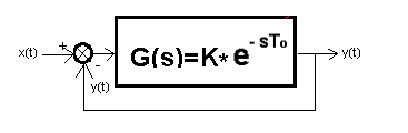
Fig.1-9
It will be found that when the K amplification is:
– K<1 then the system is stable
– K=1 the system is on the verge of stability
– K>1 the system is unstable
Fig. 1-10
An example of an unstable system when K>1
A short impulse x(t) throws the system out of balance
Isn’t this similar to the Nyquist Criterion, which will be discussed in the next chapter?
Most often we deal with multi-inertial objects in which the delay is “fuzzy”.
The principle is no longer so simple, but similar.
If in Fig. 1-9 instead of “pure” delay there will be, for example, a three-inertial unit, then we will conclude that when:
– K is small, then the system is stable
– K is average, the system is on the verge of stability
– K is large, the system is unstable
Conclusion:
High gain and inertia of the object favors instability.
Chapter 18. Amplitude-Phase Characteristics
You will learn the concept of amplitude-phase characteristics in the most natural way. You will determine it experimentally for a specific inertial unit by feeding sinusoids of different frequencies to its input.
Chapter 19. Nyquist Stability Criterion
An open system is generally stable. It can become unstable only after being closed with a feedback loop. The Nyquist Criterion can predict, based on the amplitude-phase characteristics of an open system (which is “easier” than a closed one), the stability of a closed system. Nyquist belongs to the frequency criteria.
Chapter 20. Hurwitz Stability Criterion
Unlike Nyquist, the Hurwitz Criterion is algebraic. We study the stability of the transmittance G(s) based on the coefficients of its denominator-polynomial M(s). The Hurwitz Criterion is not difficult, but quite tiring. So you can skip this topic and move on. The most important thing about this course is everything else–>chapters 21…31.
Chapter 21. On-Off Control
The control algorithm is very simple.
When the output signal y(t) is:
–greater than the set value x(t) then reduce the control signal s(t)
–smaller of the set value x(t) then increase the control signal s(t)
Fig. 1-11
On-Off Control with z(t)=+30° disturbance (additional heating).
For up to 35 seconds, the system tries to maintain the temperature around the set value x(t) = +50°C. At 35 seconds, a disturbance occurred, i.e. additional heating z(t)=+30°C. As you can see, the disturbance has been suppressed. I.e. the average temperature y(t)=+50°C is still maintained. The heating periods when s(t)=100°C are shorter than the cooling periods s(t)=0°C.
Note:
The Fig 1-11 time chart represents the above algorithm but corrected by so-called hysteresis.
Chapter 22. Continuous Control
This type of control already provides a constant steady-state control signal from the controller and a constant steady-state output signal. You will also get tired as Mr. Continuous Controller and you will also get complexes in relation to the stupid differential amplifier that acts as a controller.
The Continuous Controller will strive for the state of equilibrium:
y(t)=Kz*x(t)
where x(t) is the unit step and Kz is the gain in Fig.1-8d.
CRÉME DE LA CRÉME THAT IS CONTINUOUS PID CONTROL Chapters 23…27
Generally, I rely on intuition when writing, for example, “the regulator thinks that something is there and reacts like this and not like that”. I am trying to explain the operation of the regulator very thoroughly. and especially what the Kp, Ti and Td settings are responsible for. Manual tuning of the regulators will certainly help here. You will be looking for the optimal* response to a unit step in the input signal either to a disturbance. The conjunction either did not appear by chance.
Don’t be intimidated by the size of chapters 23…27, but all experiences are reproducible with different parameters.
We will look for optimal settings for the objects:
– one inertial unit
– two inertial unit
– three inertial unit
We will also study the effect of z(t) disturbances which will be really powerful, rather unheard of in real systems. It will be z(t)=+0.4 (heating) and z(t)=-0.4(cooling)
*There are different optimality criteria. We want the system to reach a steady state relatively quickly, even at the expense of small oscillations.
Chapter 23 P Control
You will find that this control is not accurate, there is always a control error e(t). This can be reduced by increasing the only setting of this regulator – Kp gain. Oscillations and even instability may then occur. At equilibrium, the output signal y(t) will be reached with the following value:
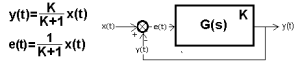
Fig.1-12
Here K=Ko*Kp is the static gain of the entire open loop, i.e. taking into account the steady-state gain of the object Ko and the gain Kp of the controller. The formulas show the steady state for the x(t) step. For large K, they approach very desirable in automatics formulas:
– y(t)=x(t)
– e(t)=0
Then the output signal y(t) mimics the input signal x(t) in steady state, or what comes to the same thing, we have zero error e(t).
Fig.1-13
Example of P control with negative disturbance z(t)=-0.2
See how the disturbance z(t)=-0.2 is suppressed. That is compenasated by additional heating in s(t) control signal. But you can always choose Kp and Td so that it is the other way around. I.e. It responds quickly to z(t) but slower to x(t).
Note that the control error is not zero as is typical for proportional control.
Chapter 24 PD Control
It gives the same control error as the P-control, but the differentiating component D greatly improves the dynamic properties. It reduces oscillations and successfully fights instability. You’ll find out in a moment.
Fig.1-14
Example of PD control with positive disturbance z(t)=+0.5
I told you so? Compare with the P Control in Fig. 1-13. Non-zero static error as for P Control. On the other hand, it greatly improves the course of regulation. Here, especially per unit step x(t).
Chapter 25 I Control
Its operating algorithm is easier than the P-regulation and similar to the on-off control:
when x(t)>y(t)–>increase the control signal gradually
when x(t)<y(t)–>decrease the control signal gradually
The decrease/increase velocity is proportional to the error e(t)=x(t)-y(t). When e(t)=0, the velocity is zero, i.e. it is in a steady state. Unlike on-off control, the steady-state control signal is constant. The most important feature is zero control error in steady state. Often novice automation specialists have a problem with this. The input is zero and the output is “not zero”? I Control is very slow and hardly used in practice. It is mainly used in teaching
Fig.1-15
I control.
It does indeed reduce the error to zero. But how bovine! Compare with PD in Fig. 1-14.
Chapter 26 PI Control
The P control is fast but does not bring the error to zero, while the I control brings the error to zero but is slow. Then let’s create a combination of P and I called PI that will be fast (but not as fast as P) but brings the error e(t) to 0. We’ll start with a didactic PI that I tinkered with. It starts as P and changes to I at some point.
Fig.1-16
PI control with positive disturbance z(t)=+0.5
The steady error is zero and comes to a steady state relatively quickly.
Chapter 27 PID Control
After adding the derivative component D to the PI controller, we obtain a PID controller which:
-also reduces the error to 0:
-however, it does it much faster than PI, much less P and even “all the more” I
The D component prevents instabilities and overshoots.
At unit step each PID controller starts as PD, then the P and D components gradually decay to zero and the I component increases from 0 to steady state y(t)=x(t), in steady state it always ends up as an I controller.
Fig.1-17
Example of PID control.
Zero error and the fastest of all. The good example of the z(t) disturbance damping.
Chapter 28 Controller Settings
You learned the first method, i.e. manual, in chapters 23…27. It was mainly used to make you feel what this setting is, so that you know what the Kp, Ti, Td settings do. There are people who assemble cabinets, regulators, valves and connect it all with cables in accordance with the automation design.
There are also those who run these systems, remove assembly and software errors. They make the Control System come alive.
I do not want to claim that this is the elite of automation. This may not be correct, but some people think so. And it is these people who tune the regulators so that the system reacts as quickly and accurately as possible. Then the system works for years. It can be accurate and fast, or inaccurate and slow. And people are surprised that the product of one company is good and expensive and the other is trashy and cheap. That is why the work of piano tuners is so responsible, pardon the PID controllers tuners.
I will present some old-fashioned methods invented during World War II by a certain Ziegler and Nichols:
-Step Response method.
-Limit Cycle method.
Each is an example of a different Philosophy. The first requires a mathematical description, i.e. the Go(s) transmittance of the object. The second is only to examine the object, or more precisely to measure the period of vibration at a certain critical amplification. So she is less fussy about the exact knowledge of the object.
To finish the topic, many modern controllers (most?) have a built-in self-tuning mechanism. Observing the input and output, the controller itself changes the parameters Kp, Ti, Td. They are so smart that you better not approach without a stick. Let’s just trust that numerous doctoral and postdoctoral theses written in the PID controller software are ok.
OTHER THINGS YOU NEED TO KNOW –>29…31
There are still a few important topics that are needed to understand the essence of automation.
Chapter. 29 Disturbances Analysis
The main signal acting on the Control System is the set value x(t). But there are other so-called disturbances z(t), which are constantly scheming, as if to harm here. More precisely, so that, for example, the output temperature y(t) instead of the one set by x(t)=+100°C was, for example, y(t)=+96°C. Steady state of course!
We are only interested in the disturbance acting on the Go(s) object. Because if the disturbance z(t) acts on the regulator and adds to the set value x(t), it is scary to even think! It was as if a spy had sneaked into the enemy army’s headquarters and started issuing orders. Fortunately, it is easier to secure a headquarters than an entire army, just as it is easier to protect against disturbances a tiny PID controller than a large Go(s) object.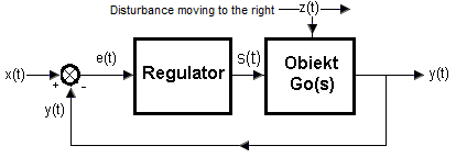
Rys.1-18
Chapter. 30 Control Systems Structures
The quality of control can be improved not only by tuning the PID, but also by changing the structure of the control system.
Typical Structures are:
1– Open loop
2– Open loop with the disturbance compensation
3– Closed loop
4– Closed loop with the disturbance compensation
5– Cascade control
6– Ratio control
The entire course so far has been about Open and Closed systems. Therefore, we will briefly discuss the others.
2. Open loop with the disturbance compensation
You control an electric furnace in which the main disturbance – fluctuations of the power network is easy to measure. Therefore, this disturbance should be measured, e.g. +37V of the amplitude and compensated with -37V of the amplitude. The furnace itself “thinks” that nothing has happened and you will not even see the impact of the disturbance. Note that there is no feedback here, hence the other name “feed forward” as opposed to the good old “feedback”.
4. Closed loop with the disturbance compensation
Compensated Open System does not suppress residual disturbances (which are not measured). So the whole thing should be closed with a simple feedback loop. And so the main disturbance-network fluctuactions be suppressed very quickly by compensation, and the remaining ones will be slowly suppressed by ordinary feedback.
Another name for this control system is Closed-Open.
5. Cascade control
This control is when it is possible to isolate a certain part of the object affected by the disturbance. And in this it is similar to the previous one – Closed loop with the disturbance compensation. However, it is not necessary to measure the disturbance. So this part can be closed with an internal feedback loop with a separate slave controller. An ordinary P controller is often sufficient here. We close the whole thing with an external loop with a master controller – most often of the PID type. Note that the P controller will quickly suppress the disturbance in the inner loop before the information about it reaches the PID controller through the large inertia of the remaining part of the object. The PID controller suppresses all other disturbances, including any imperfections in the damping of the P controller.
The principle is therefore similar to the operation of a company in which the President-master regulator suppresses all disturbances and the Manager-slave controller suppresses only “private” disturbances of his department. A good manager will suppress them so quickly that it often doesn’t reach the CEO.
And rightly so, because Mr. President, he is responsible for great matters.
6. Ratio control
Example. The color of a given paint depends on the ratio of its 2 basic components. So, fill the mixing tank with 2 flows of different paints, the flow ratio of which is constant regardless of disturbances.
Chapter 31 Effect of Nonlinearity on Control
So far we have studied linear systems. In them, the PID controller can give as much signal as it needs for fast operation. In the course, you will repeatedly encounter a situation where the furnace needs, for example, 1 kW to reach the temperature y(t)=+100°C in a steady state. But in transient states PID gives short spikes even after 1000 kW, in order to quickly reach these +100 ° C.
Real systems have limitations. The furnace can only give a maximum of 3 kW, more would be economically unjustified. It is known that the answer y(t) in this particular case of 3 kW will not be so good. But will it be much worse?
The answer to this question is precisely the purpose of this chapter. It is also to show that the main non-linearity negatively affecting the quality of regulation are the limitations of the Power Amplifier. This amplifier also has another name – Final Control Element.